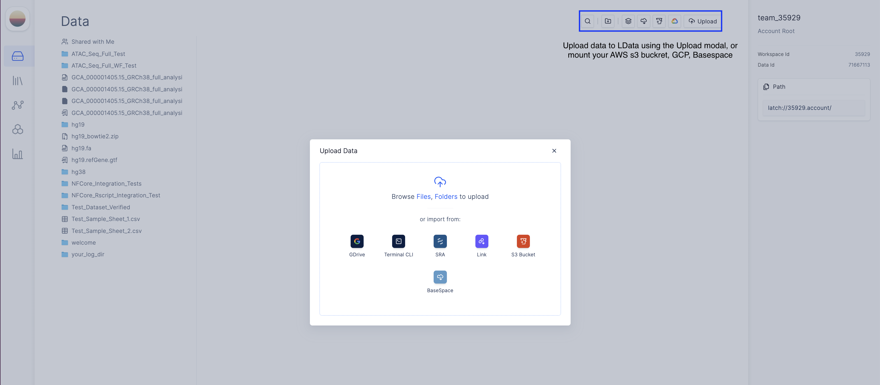
Upload your ATAC Seq data
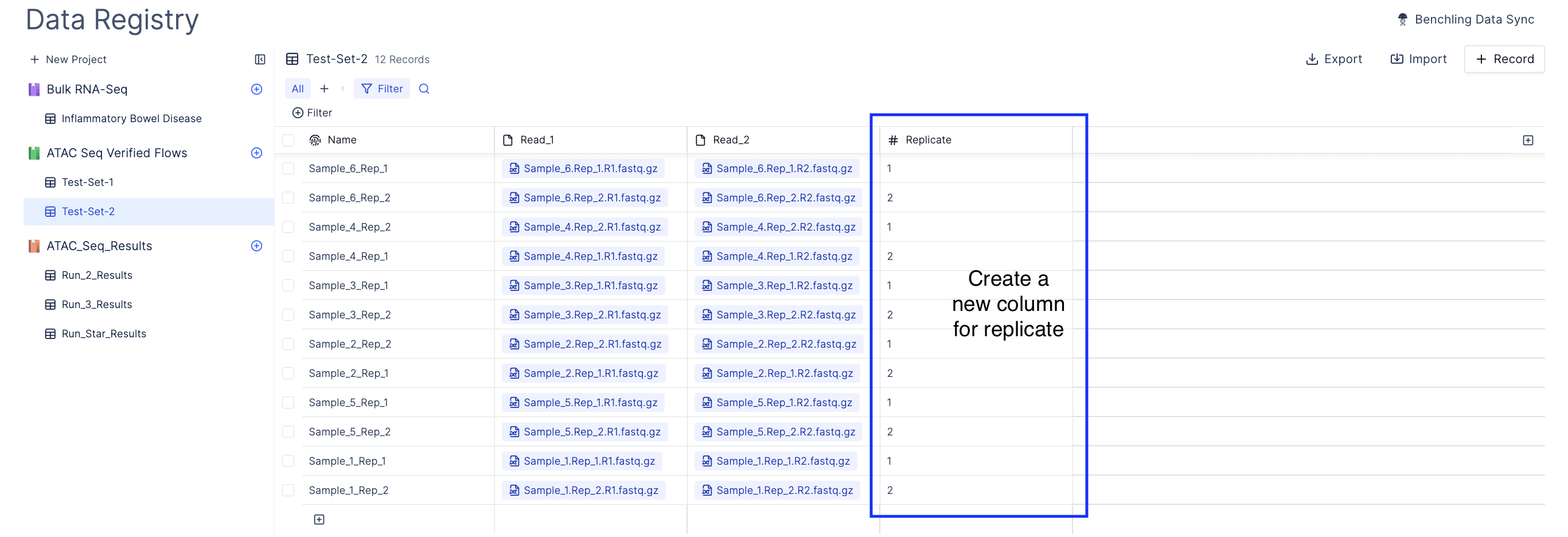
Set up sample sheet on Latch Registry
- Navigate to the Latch Registry tab on the left panel
- Create a new table.
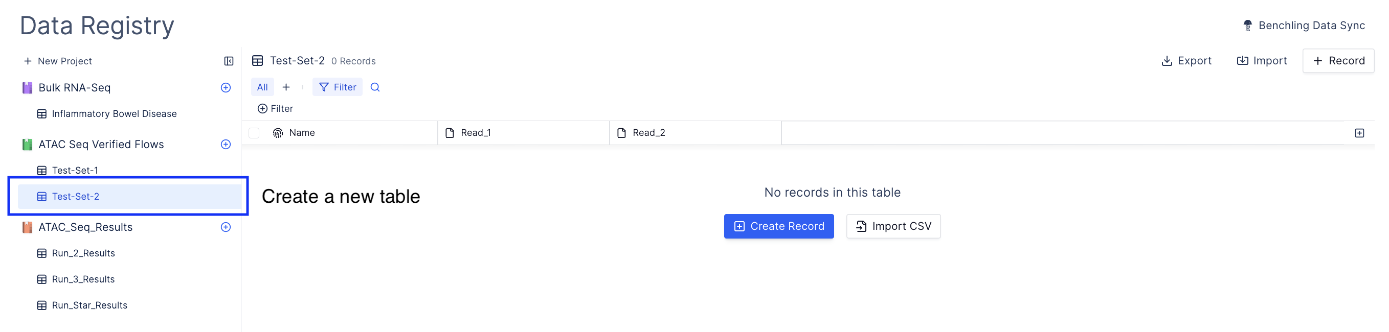
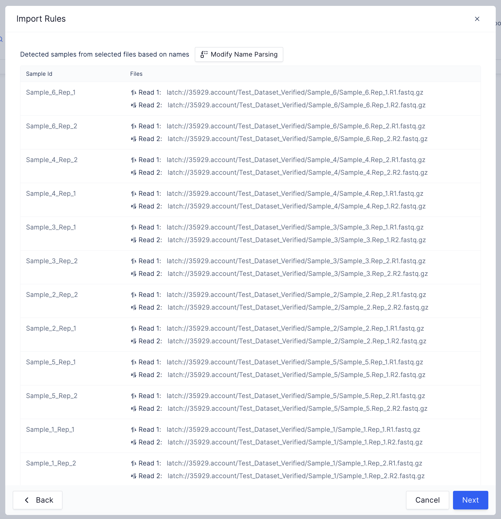
Bulk import sequencing run.
Navigate to import and select Bulk Import Sequencing Run and navigate to the directory containing sequencing data.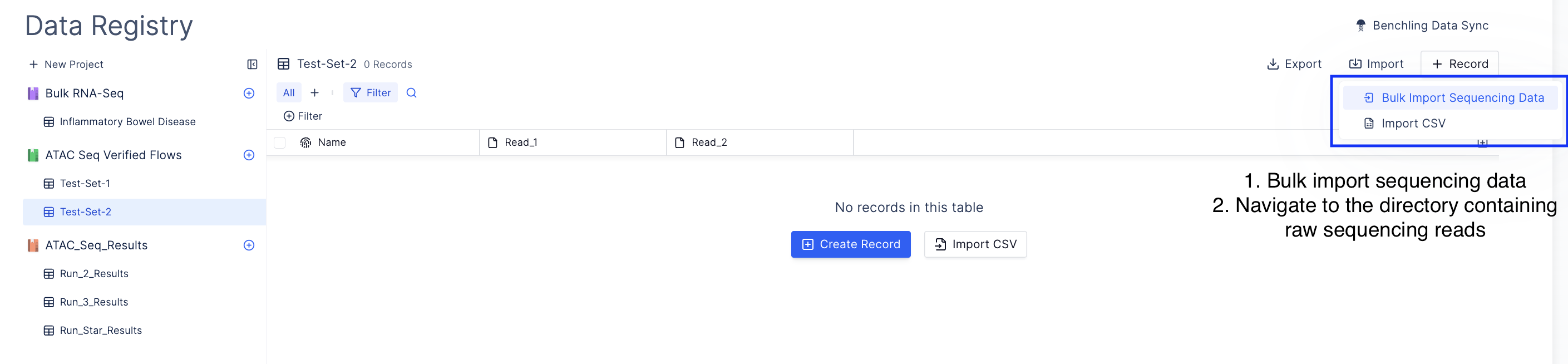
Launch NFCore/ATACSeq Workflow
- Navigate to the Latch Workflows tab on the left panel.
- Choose the ‘nf-core/atacseq’ workflow in ‘All Workflows’ or My Workflows’ (if you have added it).
-
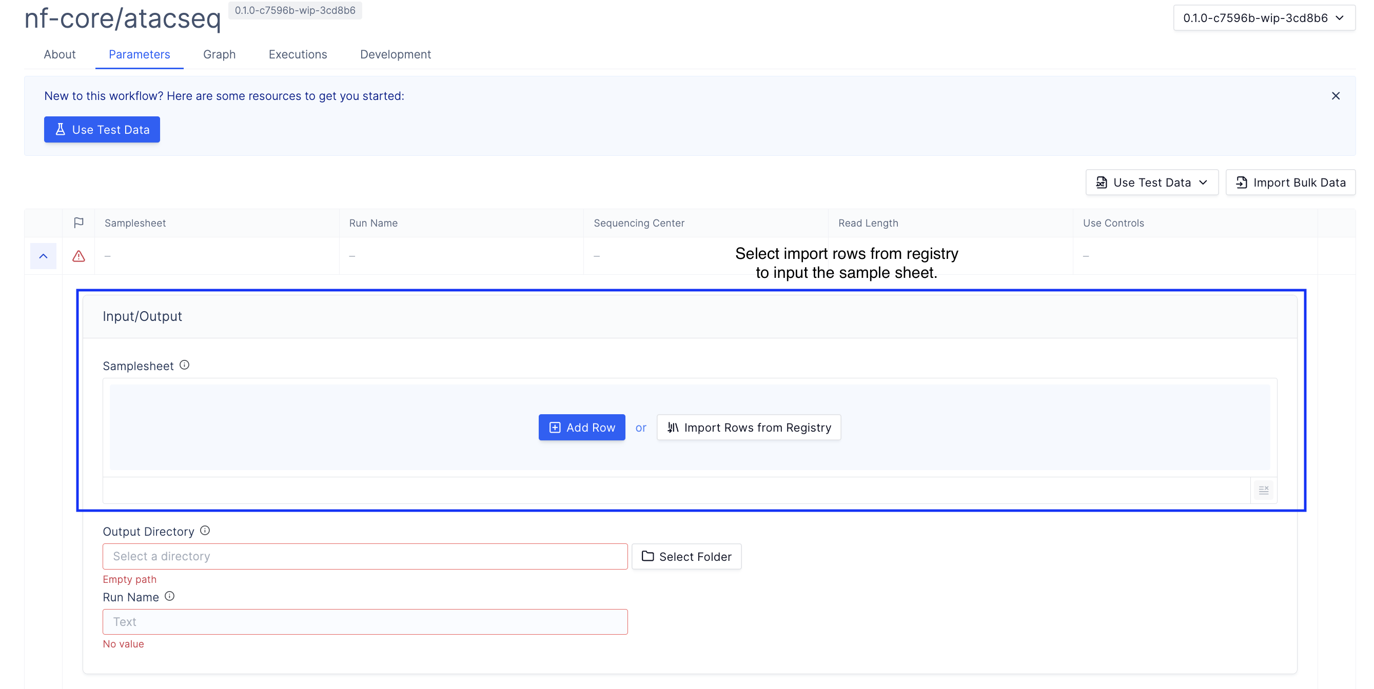
Import rows from the registry.
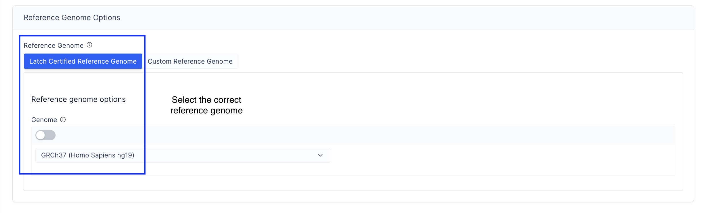
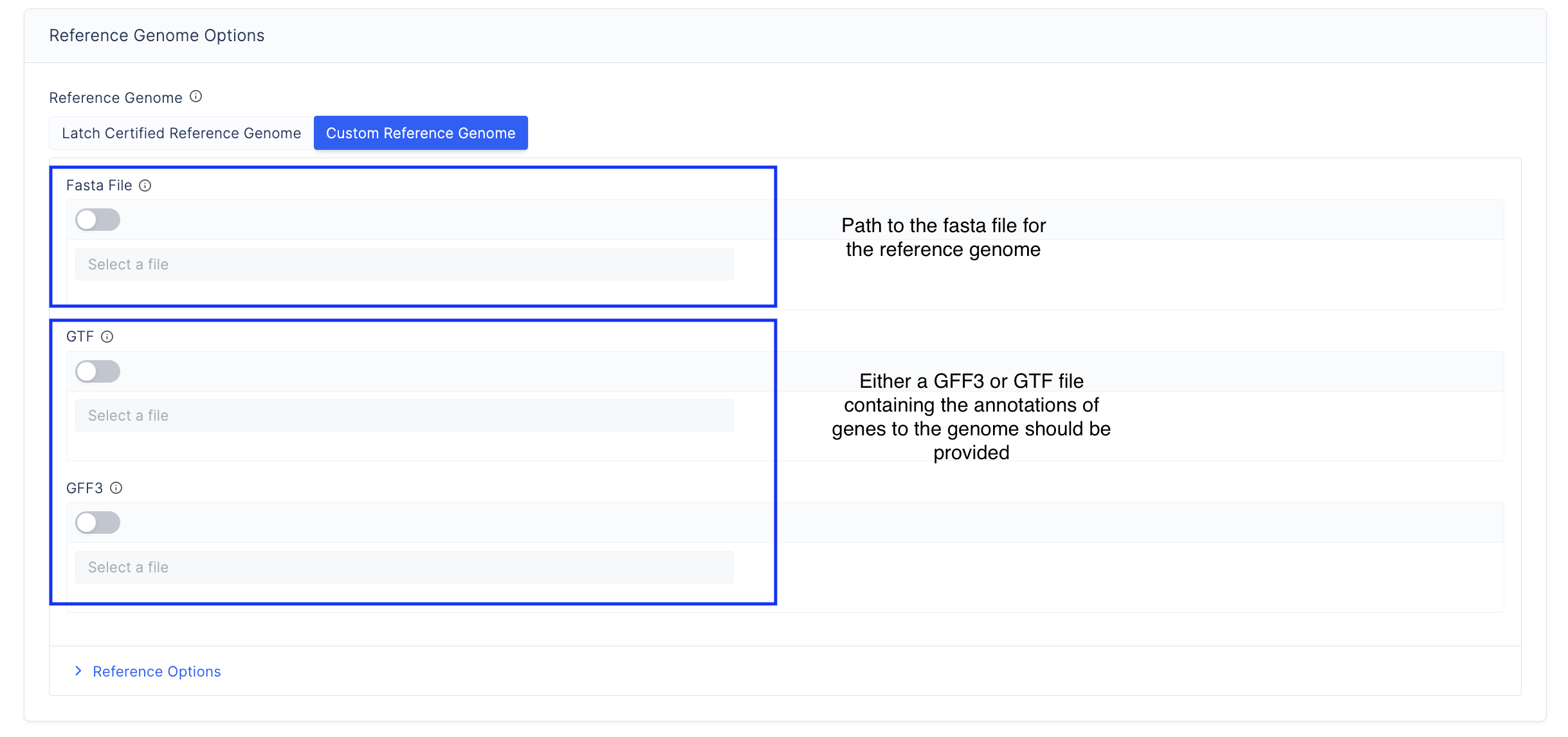
- Specify the reference genome. Choose from the latch-verified custom reference genome or input your own reference genome.
-
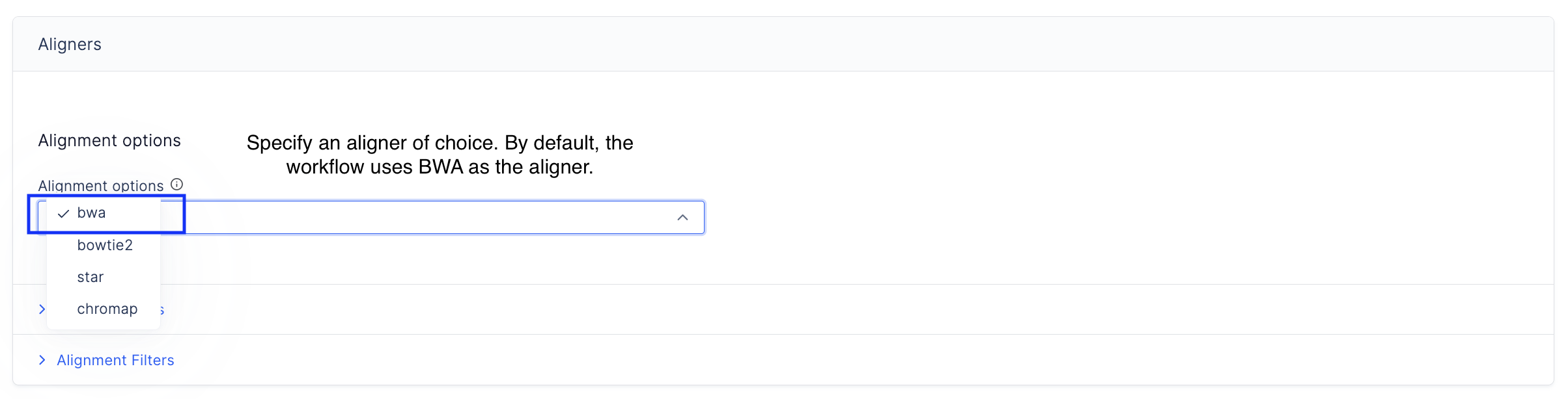
Specify the aligner used to align reads to the reference genome.
-
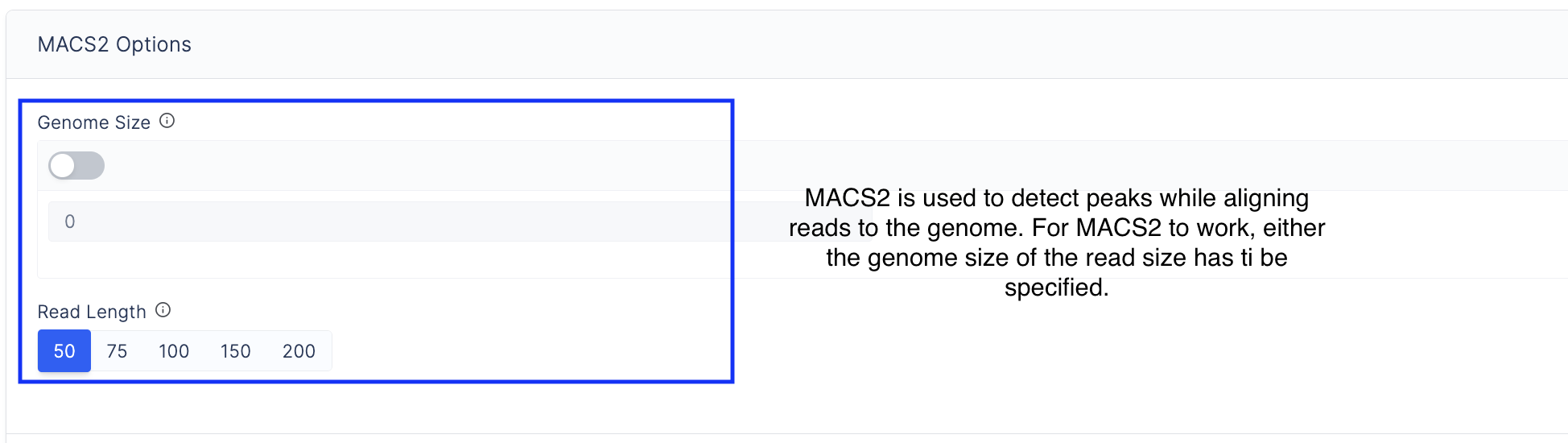
Specify options used to run MACS2, which is a peak calling software.
-
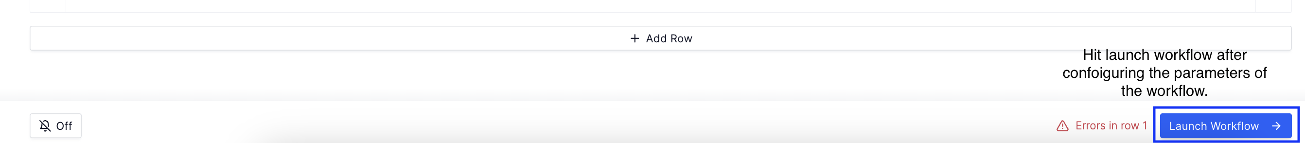
After configuring the workflow parameters, hit launch workflow
Results from running the NFCore/ATACSeq workflow
Key Takeaways
- The results from the ATAC Seq library preparation are available in the [output directory]/[run name] on ldata
- The workflow produces alignments, peak files, bigwig files that can loaded into IGV, and peak annotations with HOMER.
- Sample level analysis can be found at,
- The peak files are found at [output directory]/[run name]/[aligner name]/merged_replicate/macs2/broad_peak/[sample id].mRp.clN_peaks.xls
- The peak annotations are found at [output directory]/[run name]/[aligner name]/merged_replicate/macs2/broad_peak/[sample id].mRp.clN_peaks.annotatePeaks.txt
- The bigwig files that can be viewed with IGV can be at [output directory]/[run name]/[aligner name]/merged_replicate/macs2/bigwig/[sample id].mRp.clN.bigWig
- Replicate level analysis can be found at,
- The peak files are found at [output directory]/[run name]/[aligner name]/merged_replicate/macs2/bigwig/[sample id].mRp.clN_peaks.xls
- The peak annotations are found at [output directory]/[run name]/[aligner name]/merged_replicate/macs2/bigwig/[sample id].mRp.clN_peaks.annotatePeaks.txt
- The bigwig files that can be viewed with IGV can be at [output directory]/[run name]/[aligner name]/merged_replicate/macs2/bigwig/[sample id].mRp.clN.bigWig
- Results from running differential accessibility analysis can be found here at,
- Results from PCA can be found here at, [output directory]/[run name]/[aligner name]/merged_library/macs2/broad_peak/consensus/deseq2/consensus_peaks.mLb.clN.pca.vals.txt
- The PCA distance matrix is available here at, [output directory]/[run name]/[aligner name]/merged_library/macs2/broad_peak/consensus/deseq2/consensus_peaks.mLb.clN.sample.dists.txt
Supplementary Results
- The intermediate alignments, fastqc reports, multiqc reports, genome information, and the trimmed read information is available here at, [output directory]/[run name]/[aligner name], [output directory]/[run name]/fastqc, [output directory]/[run name]/genome, [output directory]/[run name]/multiqc, and [output directory]/[run name]/trimgalore
- The pipeline also creates two other directories namely [output directory]/[run name]/R_Plots and [output directory]/[run name]/cov_parquet/ that hosts the data matrices required for plotting results with the Latch Verified ATACSeq Plots layout.
Sample registry tables
Further, the workflow creates a table in the registry with the run name within the project “ATAC_Seq_Results”. This table carries data tables computed as a part of the workflow that can be loaded with the verified ATAC Seq plots layout, which helps visualize the results from the workflow.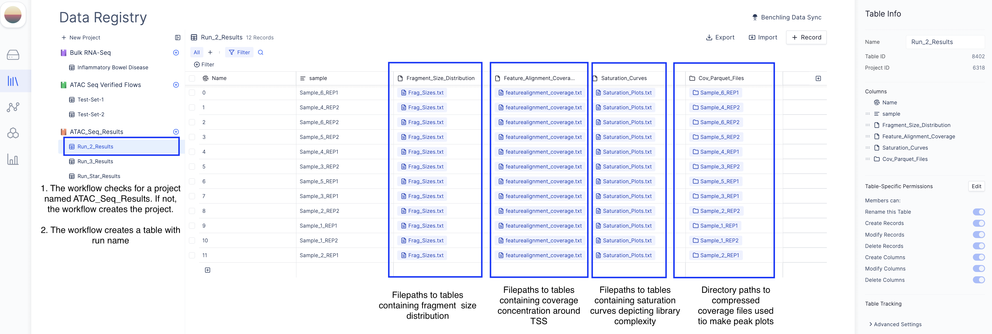
Plotting Layout
-
Create a new plotting template by choosing the Verified ATAC Seq Plots Layout from the list of available plots layout,
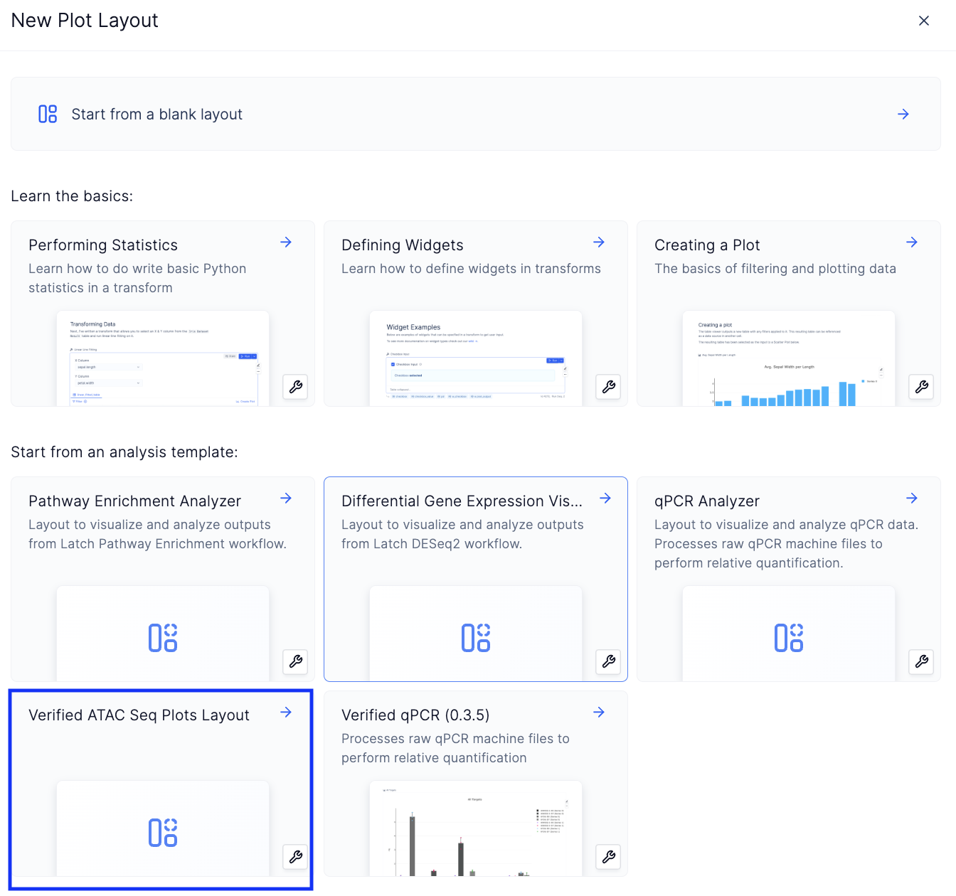
Create a new plots layout
Load a template
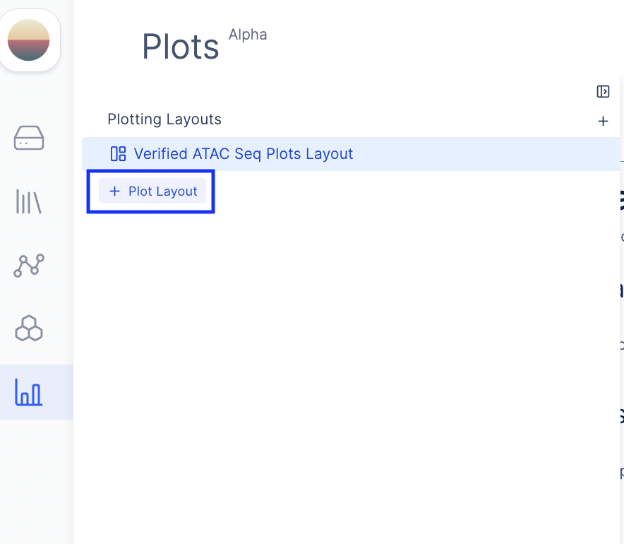
Verified ATAC Seq Layouts
-
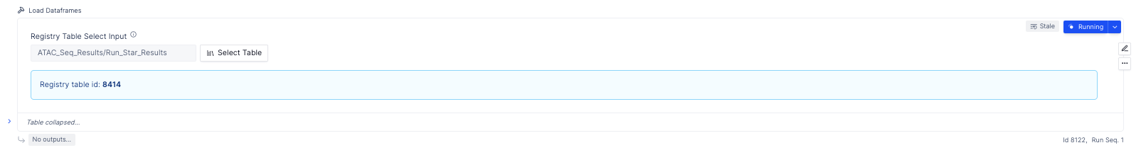
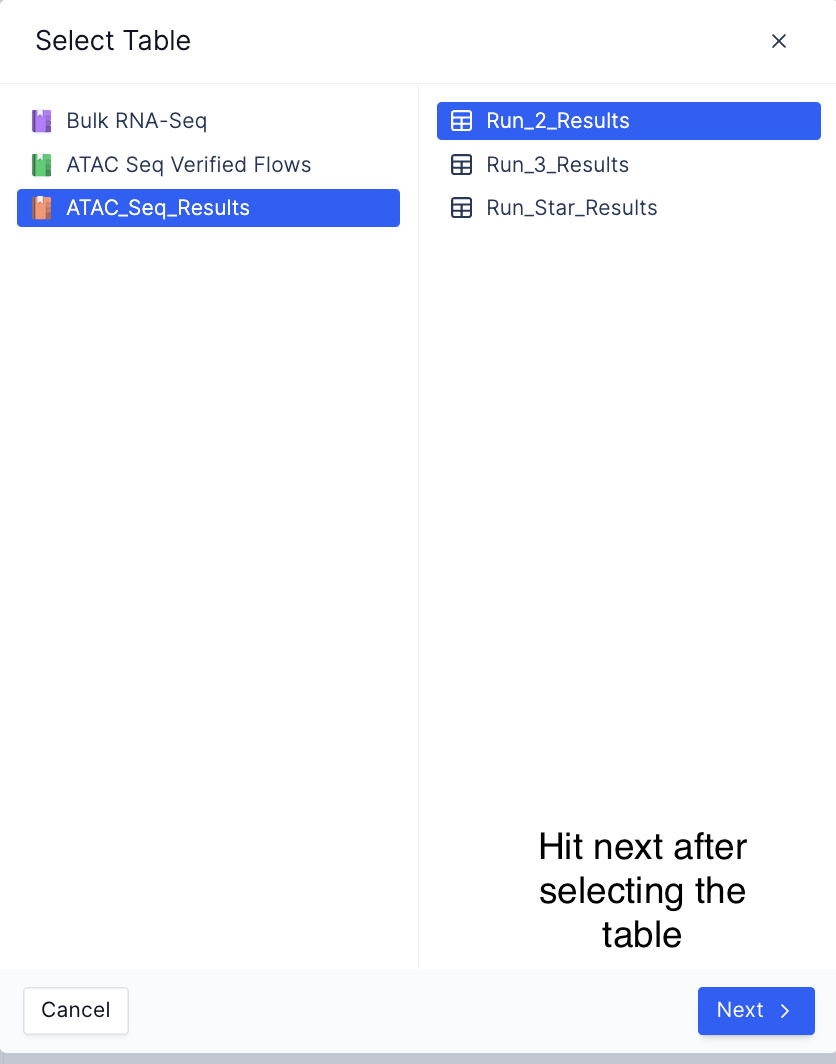
Load the data matrices by loading the registry table created as a part of the workflow,
Load registry table from the select table widget
Select project modal
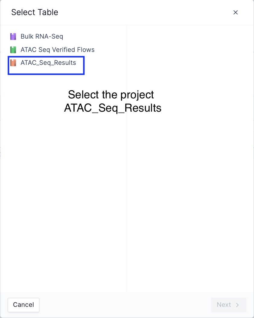
Select table modal
-
The plotting layout automatically loads all the dataframes needed to make plots and produces the following plots.
Distribution of fragment lengths
The distribution of fragment lengths obtained from a paired-end ATAC seq library has an inherent periodicity to it and the distribution decays exponentially. The first peak corresponds to nucleosomal regions, the second peak to mononucleosomal regions, the third peak to dinucleosomal regions, etc., This curve is characteristic of ATAC Seq libraries and is an essential step in quality control analysis. A good ATAC seq library has a clear peak with periodicity (of about 200 bases), and errors in library prep could result in the largest peak at nucleosome-bound portions, on the other hand, a sub-optimally transposed library has no visible peaks at nucleosome-bound regions. These curves often serve as a certificate of goodness for ATAC seq library preparation.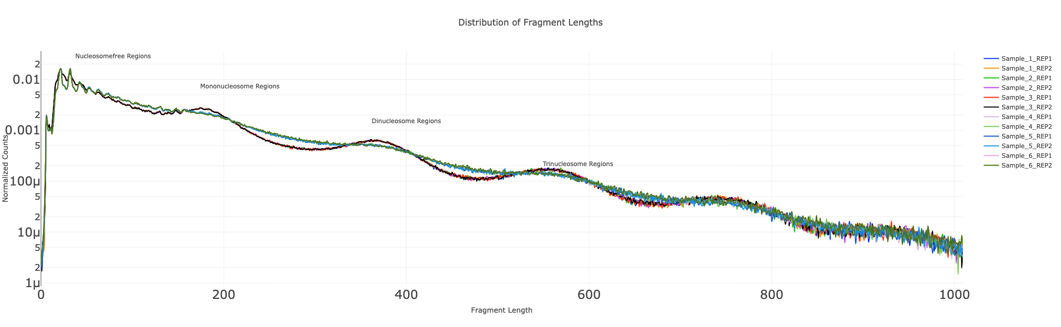
Fraction of coverage signal around Transcription Start Sites (TSS)
As described early on, the pileup of reads in nucleosome-free regions is the highest with ATAC seq libraries. Promoters of active regions typically, found in open chromatin regions of the chromosome are captured by ATAC seq libraries. Thus, fragments shorter than 100 bases are typically indicative of nucleosome-free segments. The concentration of signal immediately around Transcription Start Sites(TSS) is enriched with nucleosome-free regions. Similarly, about 200 bases from TSS, we see an enrichment for nucleosome-bound regions. We extract the signal in the TSS and disaggregate the signal from fragments with nucleosome-free and nucleosome-bound regions of the chromosome. These curves are also used in the quality control analysis of ATAC seq data. A good library would suggest that there is a larger concentration of the signal from nucleosome-free fragments near TSS.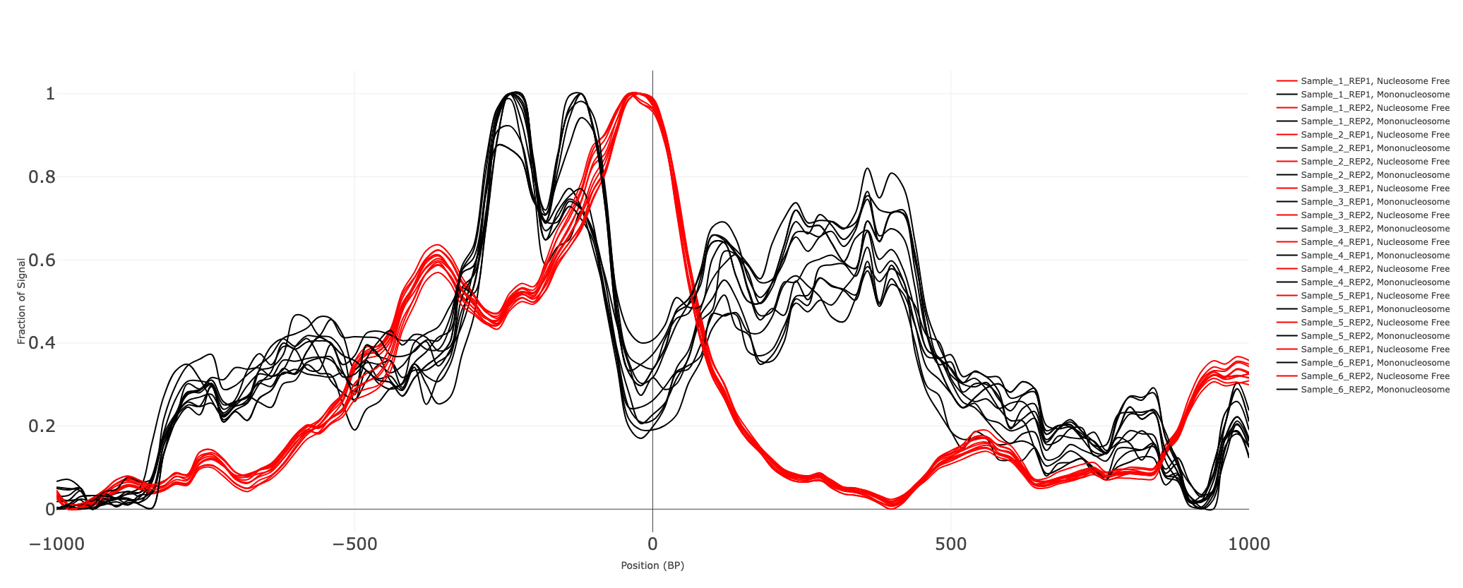
Estimating library complexity
To estimate the impact of PCR duplicates on the library preparation, we plot the number of unique fragments for different amounts of putative segments sequenced. The curves help compare biases originating from library preparation between different samples.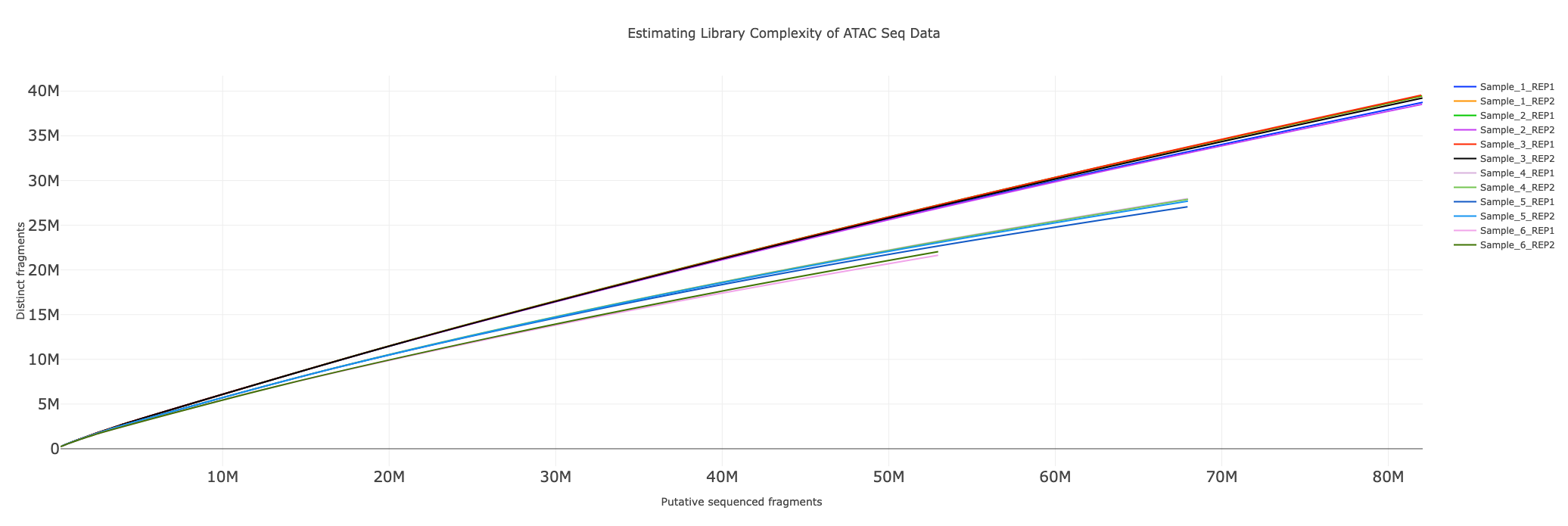
Differential Accesibility Analysis (PCA Plots)
We plot the principal component transformed “peak count” matrix as a scatter plot along the top PCs. The scatter points are also annotated with the sample names, making it immensely easy to compare between samples and replicates.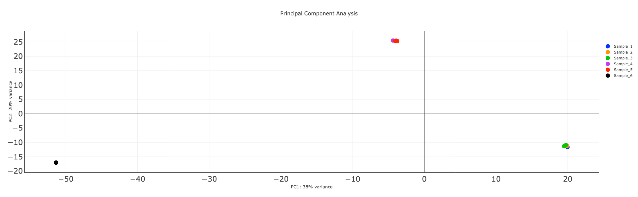
Differential Accesibility Analysis (PCA Distance Matrix)
We also plot a heatmap of the pairwise distances which provides an alternate view of the same data.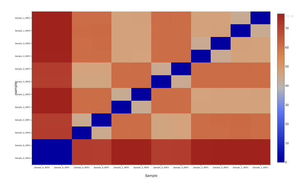
-
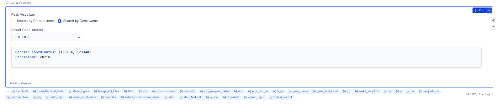
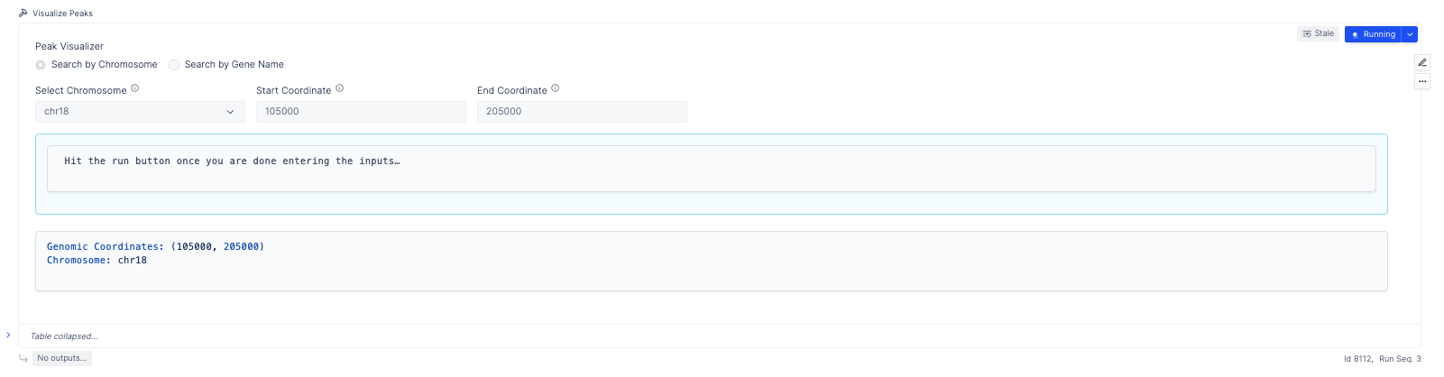
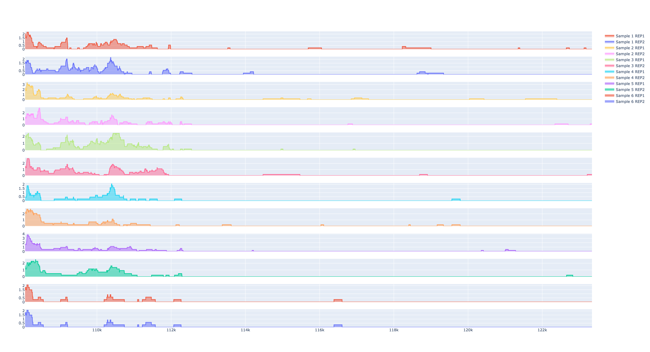
The plotting layout further makes it very easy to visualize peaks across samples, and provides functionality to search by genes and chromosomes.
Visualize Peaks
The ATAC seq peaks constitute the most important aspect of the analysis of ATAC seq data. Conventionally, scientists have relied upon IGV to identify these segments of interest. Here in addition, to IGV sessions, we also provide an interactive peak visualization dashboard, that allows the user to select peaks based on genes/chromosomes.