General Notes
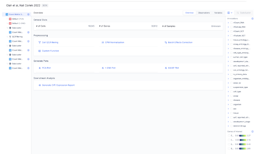
adata.obs and adata.var_names respectively. # of Samples are computed from an adata.obs.samples column if available in the file.
The AnnData file structure can be broken down into these major sections, as explained in details in the original AnnData documentation here:
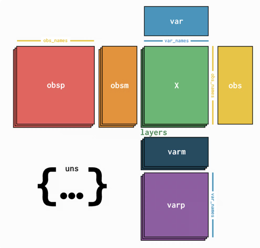
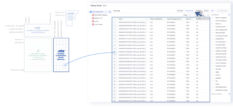
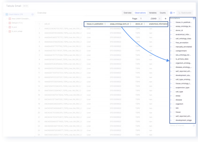
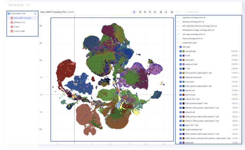
- The Observations tab maps to the
adata.obs, and the annotations on the sidebar are loaded foradata.obsas well. Any annotations that are added or edited are also added toadata.obs. Cell IDs are also loaded from the index ofadata.obs.
- The annotations on the sidebar can be used to color the UMAP, tSNE, or PCA embeddings.
- The Variables tab maps to
adata.varand the index of which (adata.var_names) are used as Gene Names by Genes of Interest and Differential Expression.
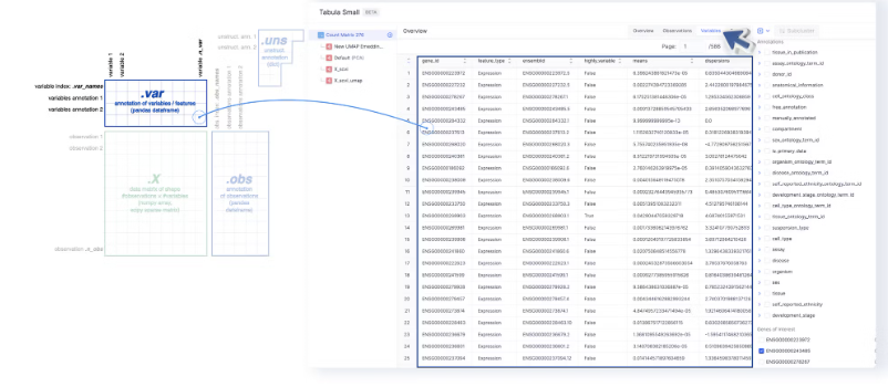
- The gene names under Genes of Interest are extracted from the
gene_idcolumn of the Variables page.
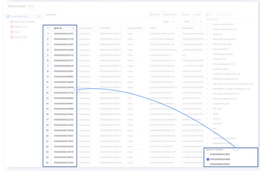
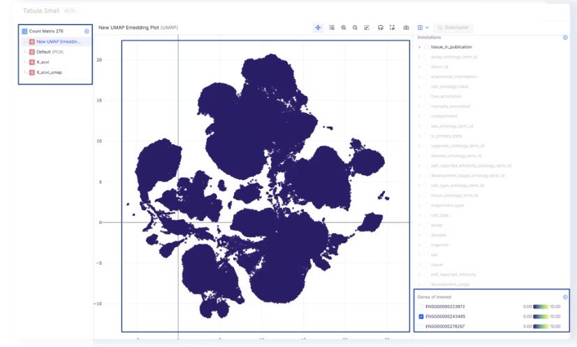
- The level of gene expression can be highlighted on the embedding by selecting one of the genes of interest.
- Embeddings are saved in
adata.obspand displayed in the visualizer. - All mutations are performed directly on the default
.Xmatrix in the AnnData file. This was done to be in spec with Latch’s Single Cell Pipeline. At the moment we do not support editing/replacing layers in the visualizer. Instead, each AnnData file is immutable, any operations that strictly mutates the underlying counts/.X matrix create a new node (.h5ad file)
Mutations
The Single Cell Visualizer contains a series of mutations that can be run on each AnnData file. The frontend passes the selected parameters to ascanpy function on the backend, which subsequently runs the mutation.
An example of how this looks:
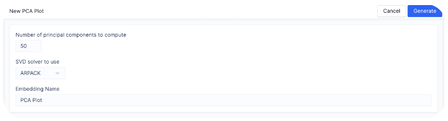
n_comps
and svd_solver parameters of scanpy.tl.pca. Note that if there are no exposed parameters for a mutation on Pollock, default parameters from scanpy are used. To see an exhaustive list of default values for scanpy functions, visit Scanpy API reference here.
A list of mutation names on Pollock and underlying Scanpy functions is provided below.
| Mutation Type on Pollock | Mutation Name on Pollock | Underlying Scanpy Function |
|---|---|---|
| Cell QC/ Filtering | Counts | scanpy.pp.filter_cells |
| Cell QC/ Filtering | Detected Genes | scanpy.pp.filter_genes |
| Cell QC/ Filtering | Mitochondrial Counts | scanpy.pp.calculate_qc_metrics (for genes detected with prefix MT-) |
| Cell QC/ Filtering | % Ribosomal Counts | scanpy.pp.calculate_qc_metrics (for genes detected with prefix either RPS or RPL) |
| Normalization | CPM Normalization | scanpy.pp.normalize_total |
| Log Transform | Log Transform | scanpy.pp.log1p |
| Batch Correction | Scanpy | scanpy.pp.combat |
| Batch Correction | Harmony | scanpy.external.pp.harmony_integrate |
| PCA (Inplace) | PCA | scanpy.tl.pca |
| TSNE (Inplace) | TSNE | scanpy.tl.tsne |
| UMAP (Inplace) | UMAP | scanpy.tl.umap |
| Neighbors (inplace) | Neighbors | scanpy.pp.neighbors |
| Differential Expression (Inplace) | Differential Expression Report | scanpy.tl.rank_genes_groups |
| Subclustering | Subclustering | AnnData filtering, ex: adata = adata.loc[adata.obs[cell_type] == “t-cell”] |
| Clustering | Leiden | scanpy.tl.leiden |
| Differential Expression (Inplace) | Louvain | scanpy.tl.louvain |
filter_cells and filter_genes don’t allow for concurrent filtering of cells and genes. In these cases, the functions are run with min_cells and min_genes respectively before being run again with max_cells and max_genes respectively based on the range provided via the plot.