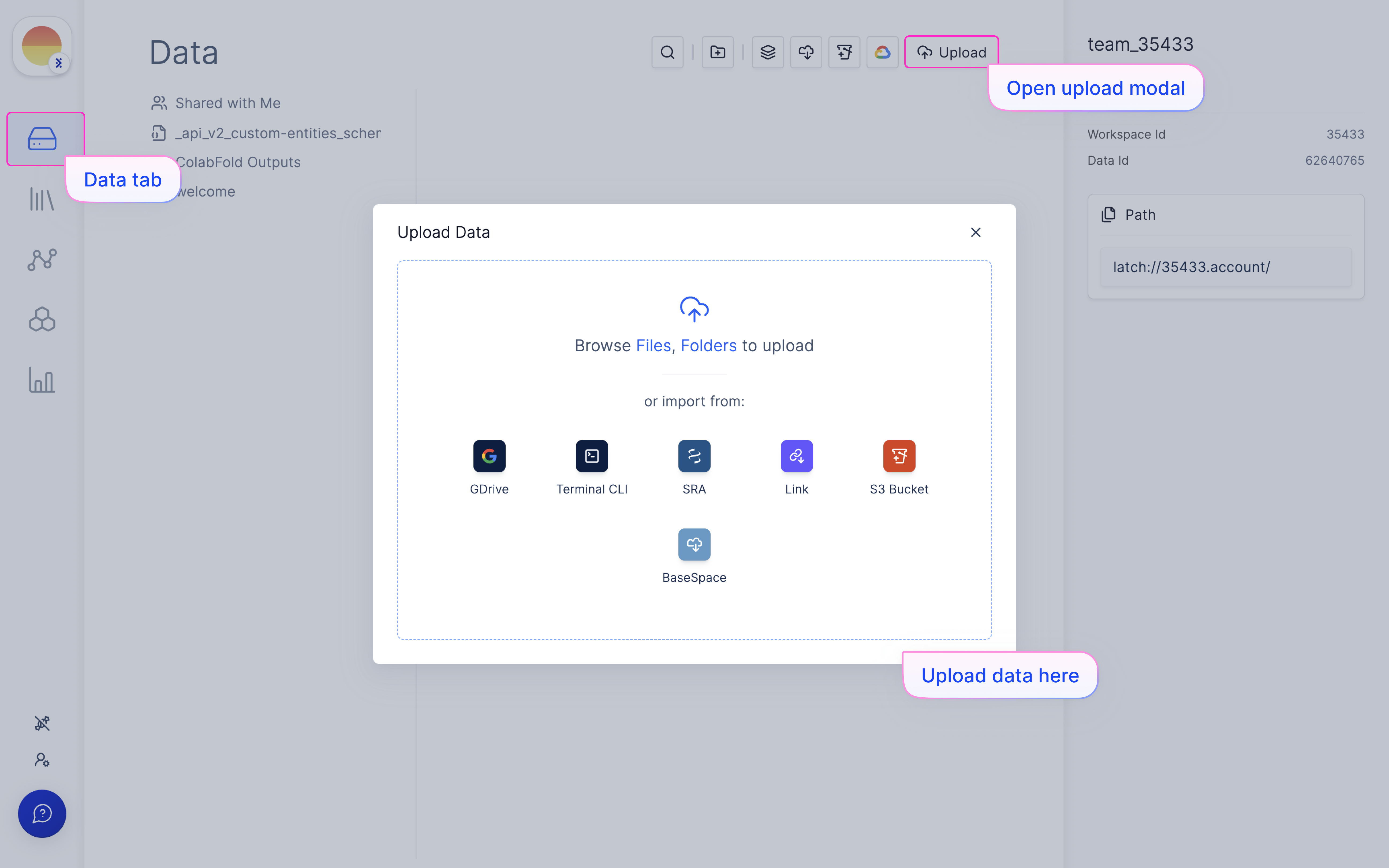
Upload your RNAseq data
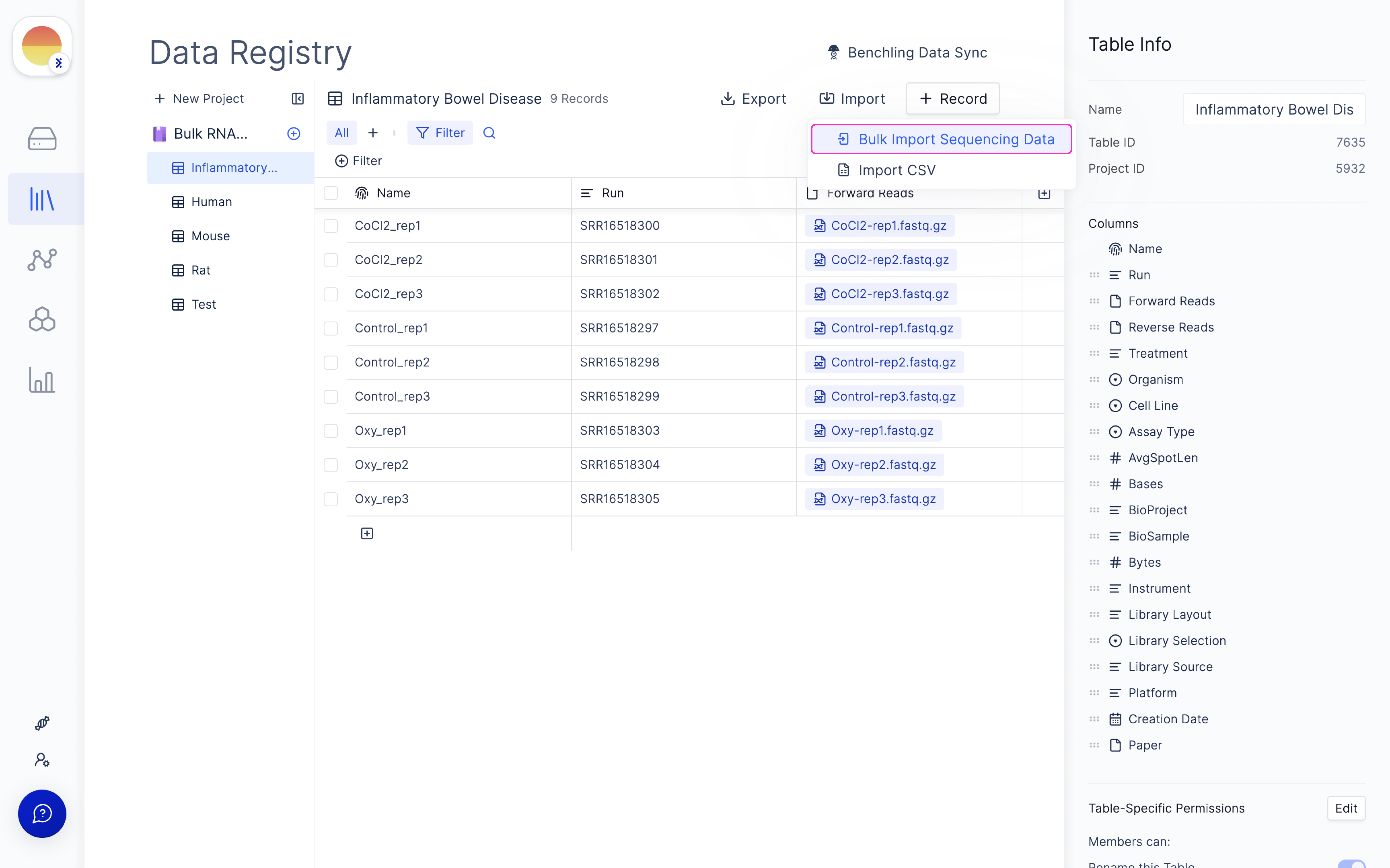
Set up samplesheet on Latch Registry
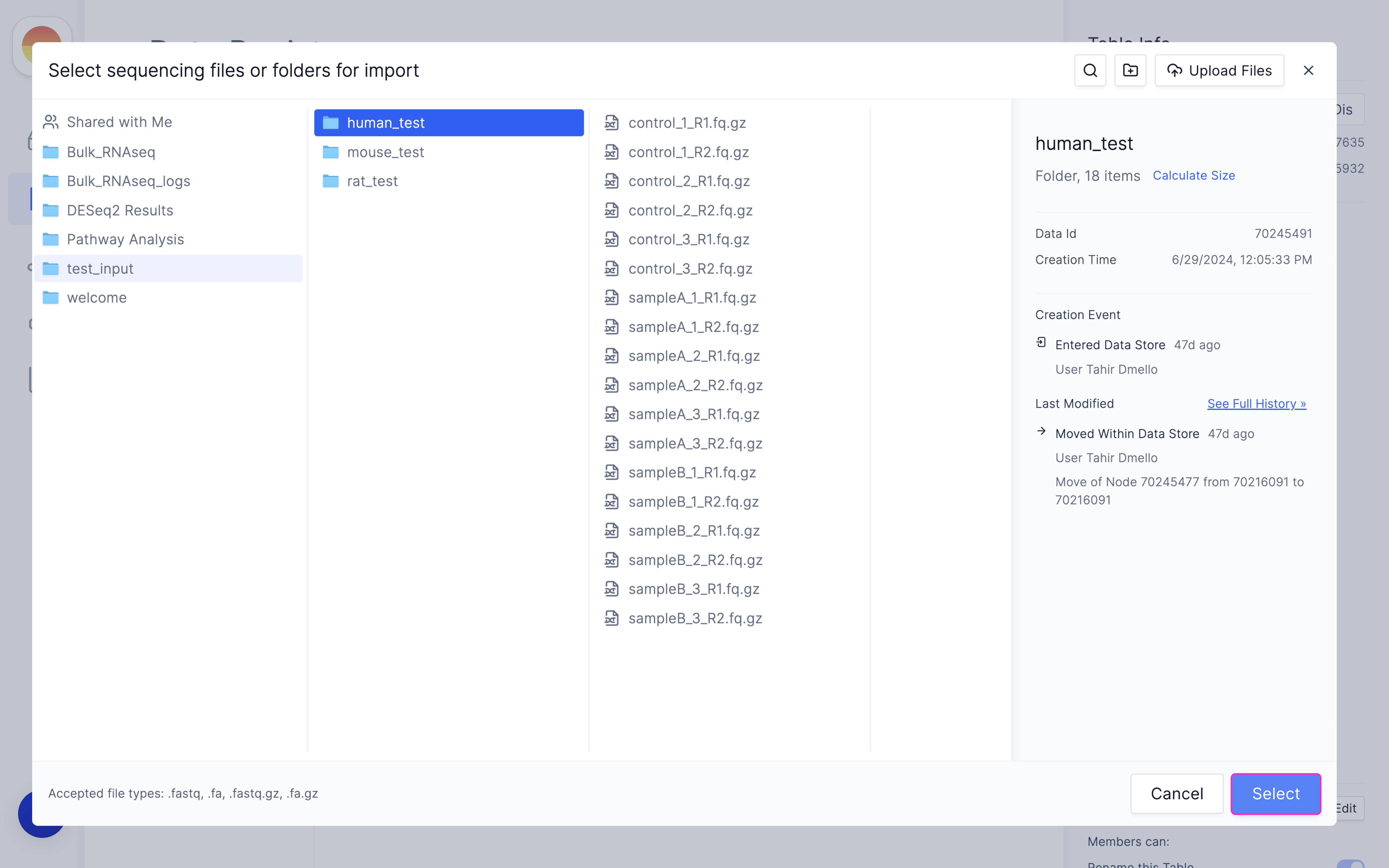
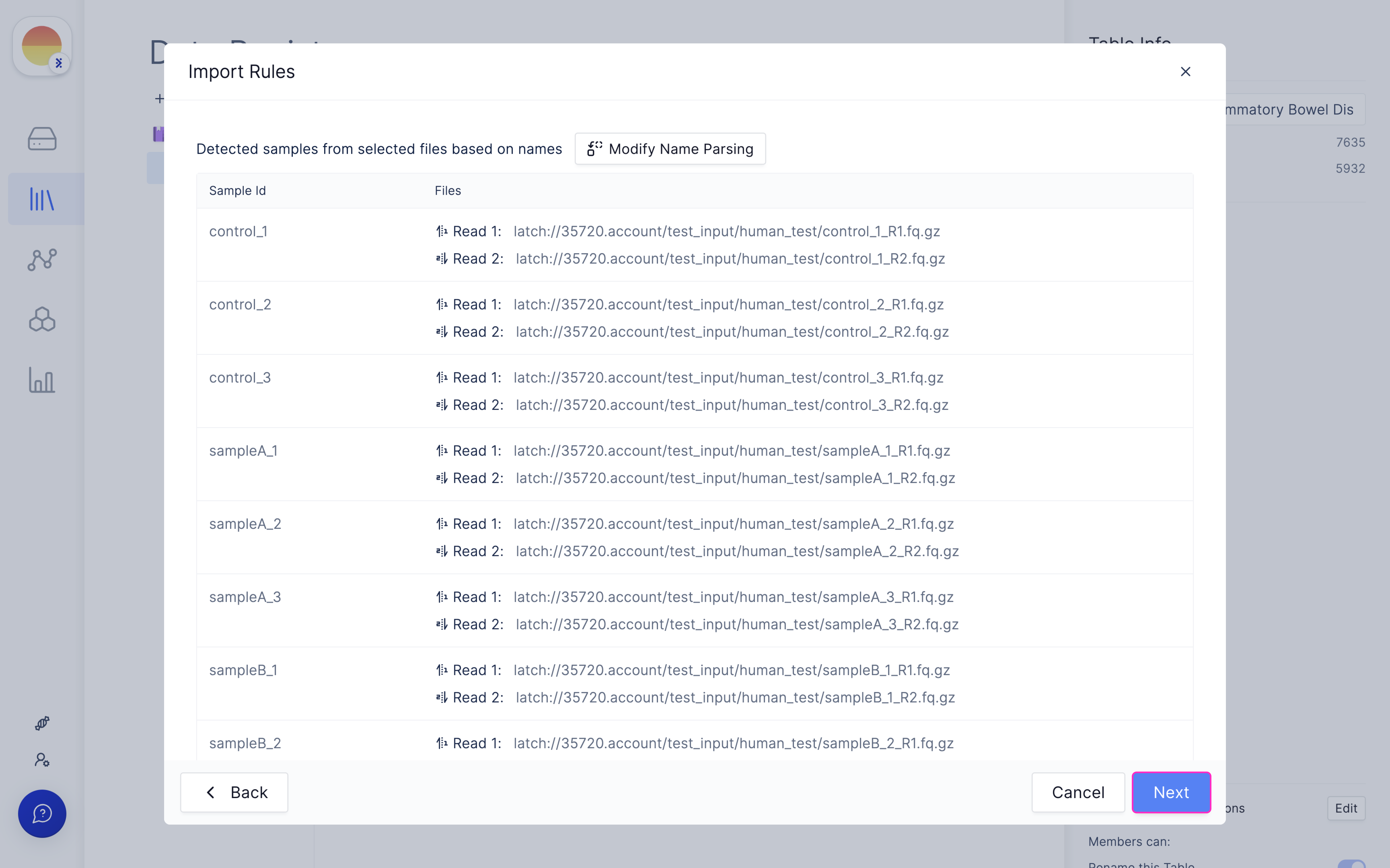
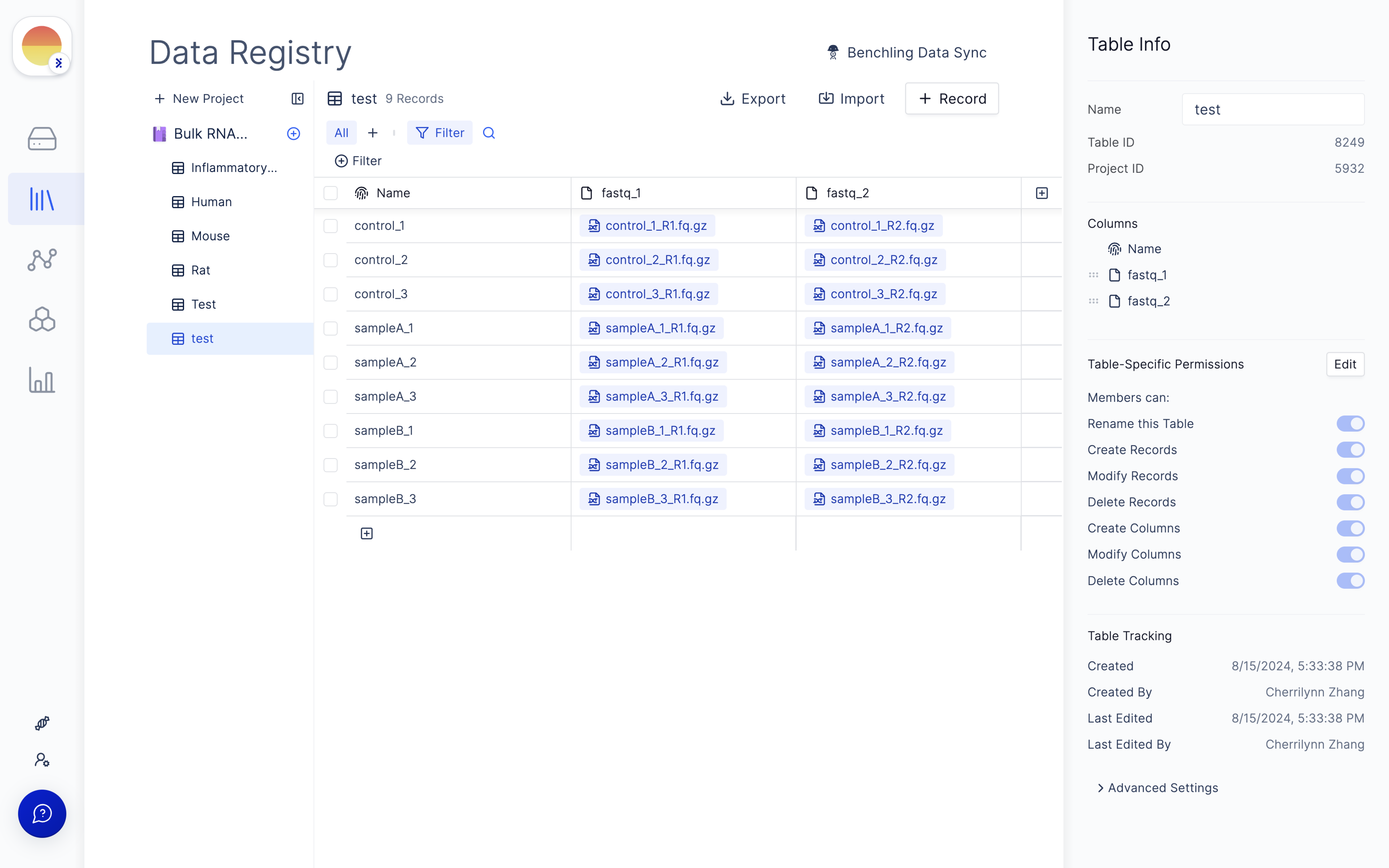
Navigate to the Latch Registry tab on the left panel.
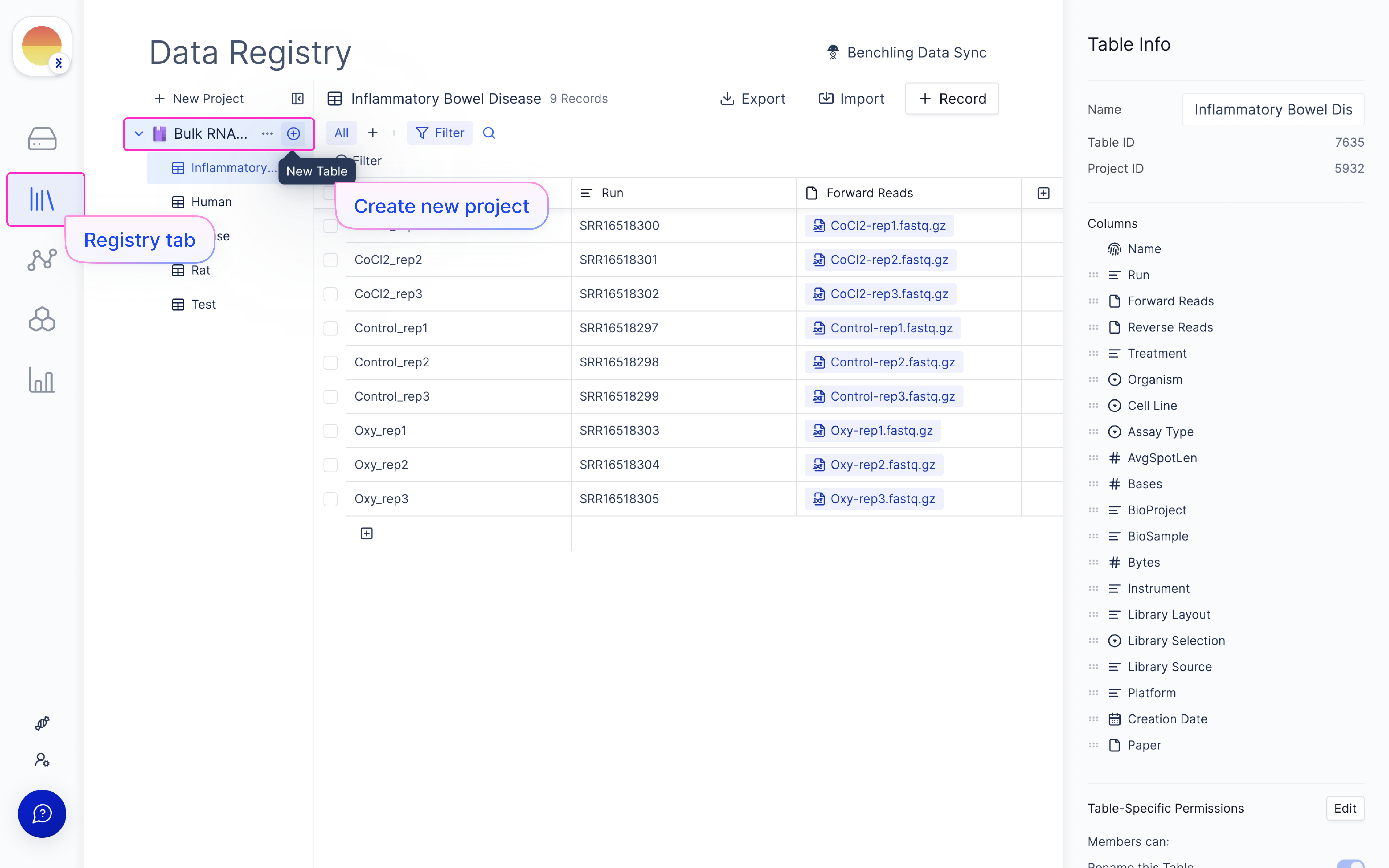
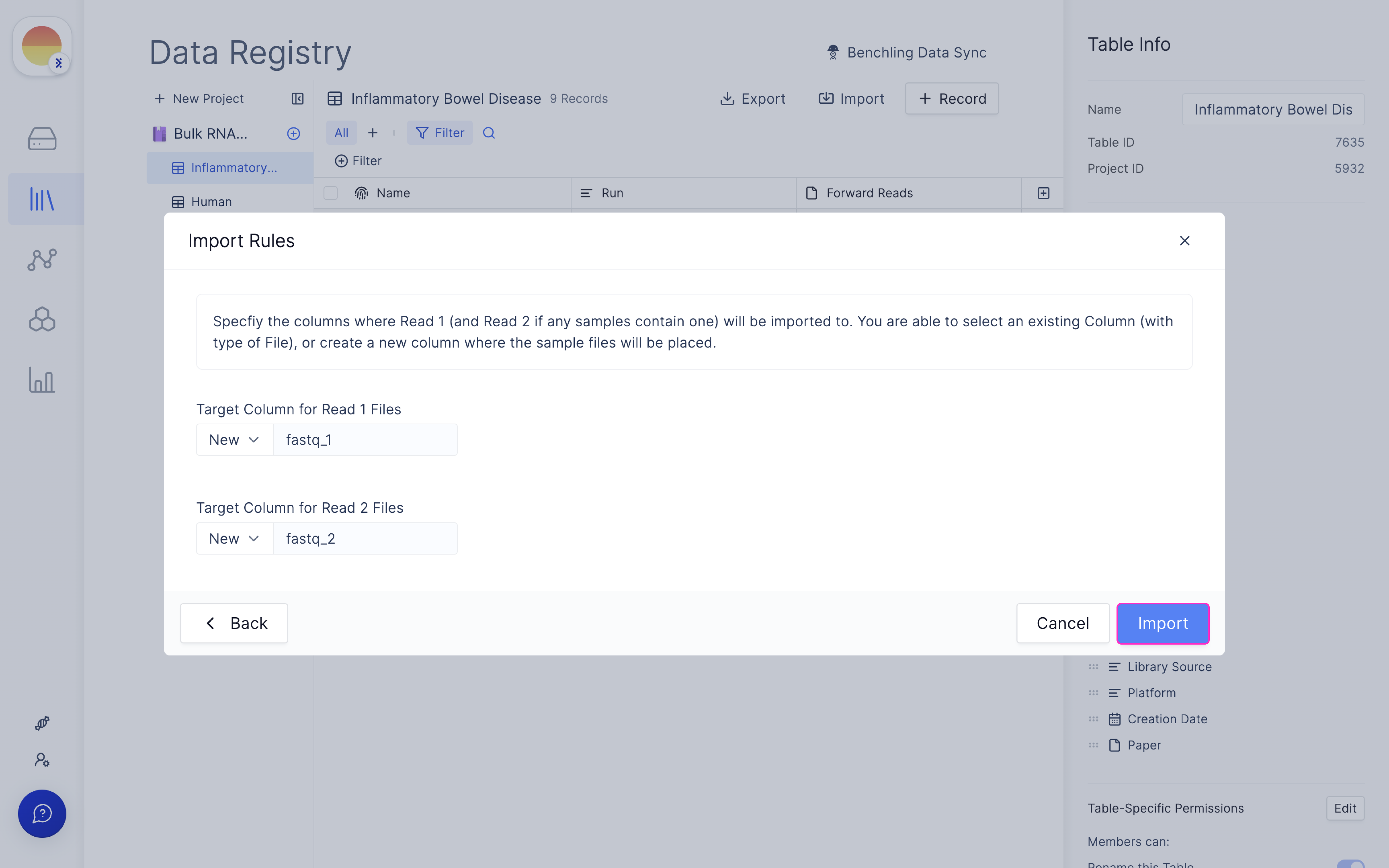
Fill in ‘fastq_1’ and ‘fastq_2’ for your forward and reverse read file respectively and click ‘Import’.
Launch ‘nf-core/rnaseq’ Latch Workflow
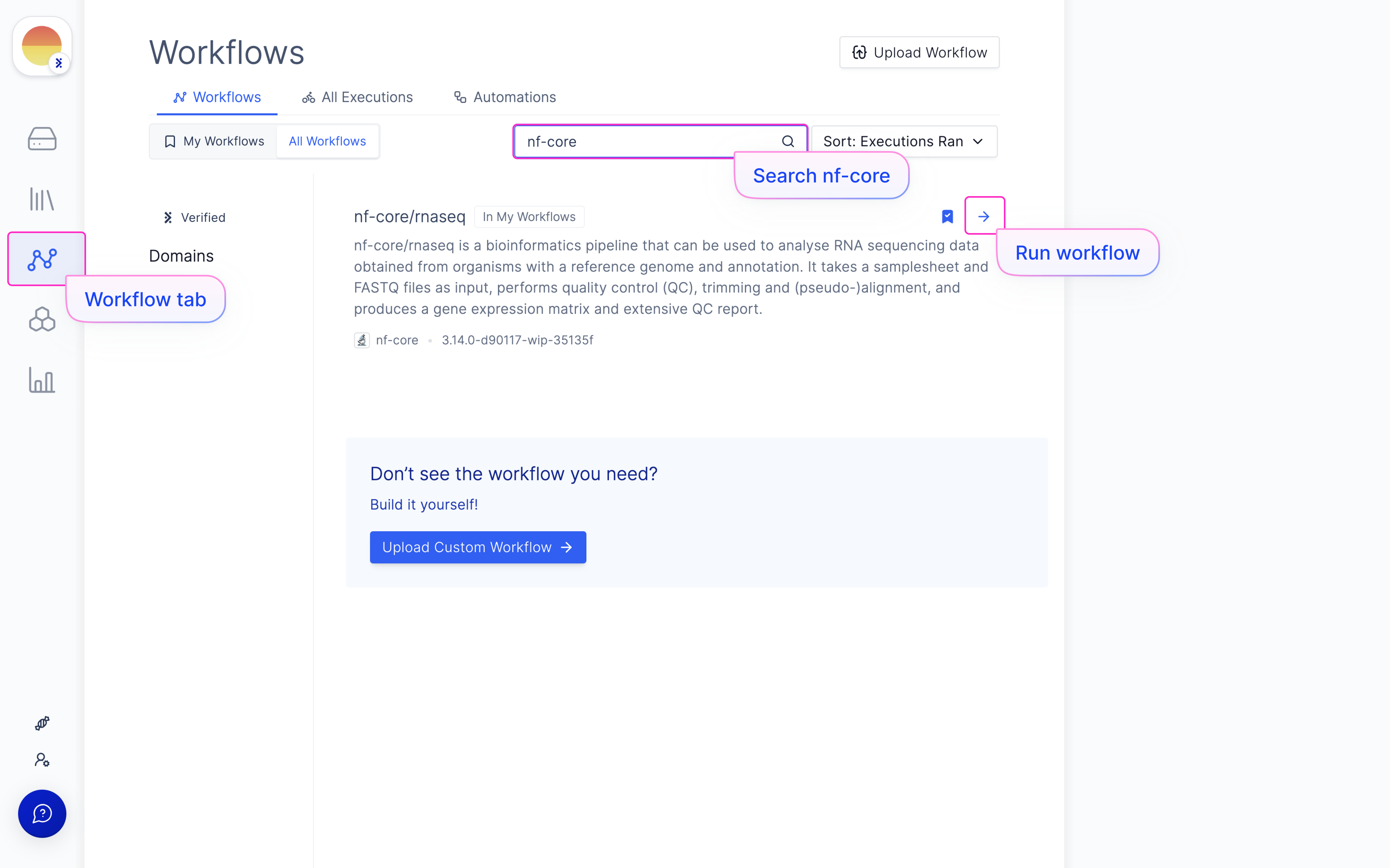
Navigate to the Latch Workflows tab on the left panel.
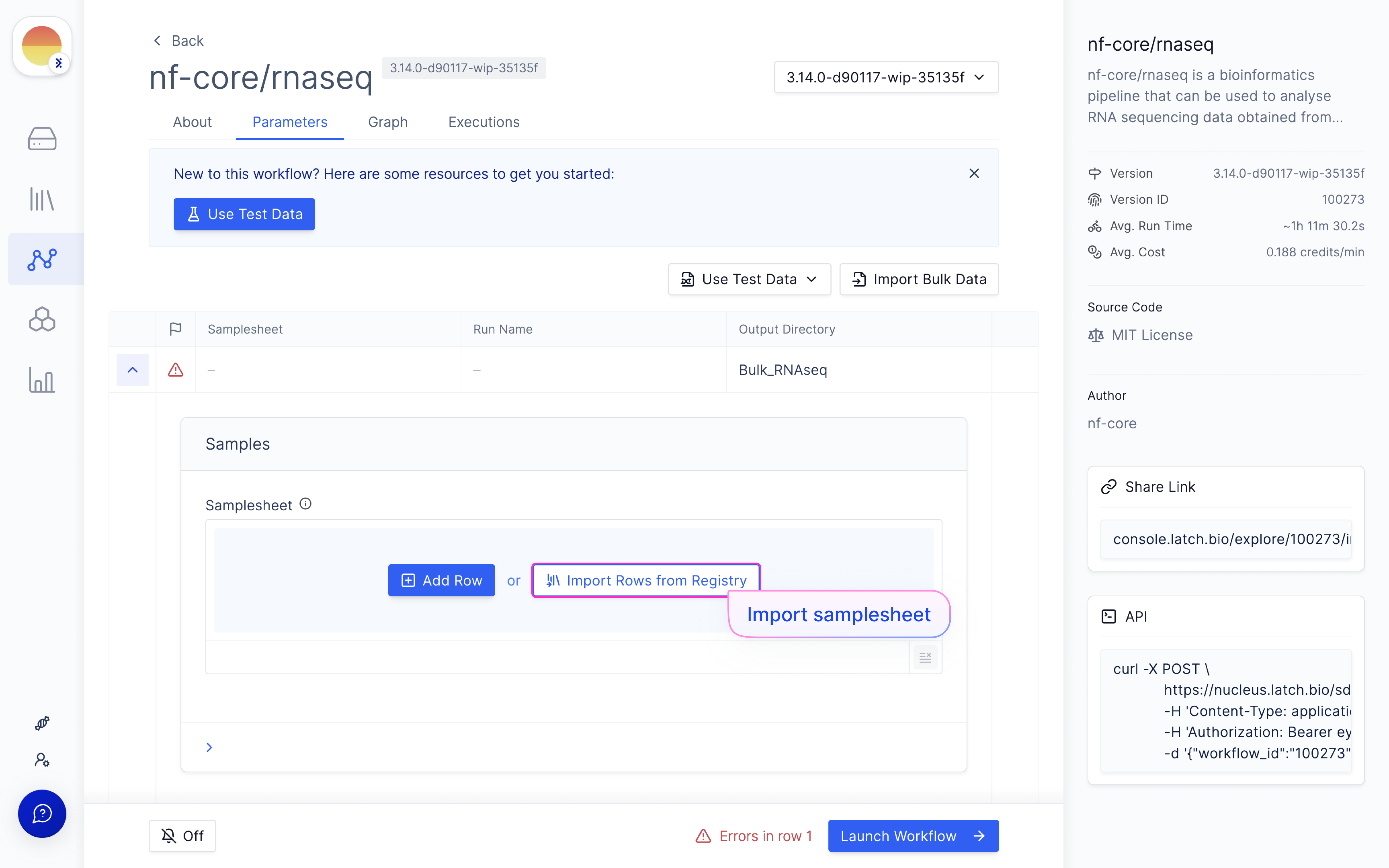
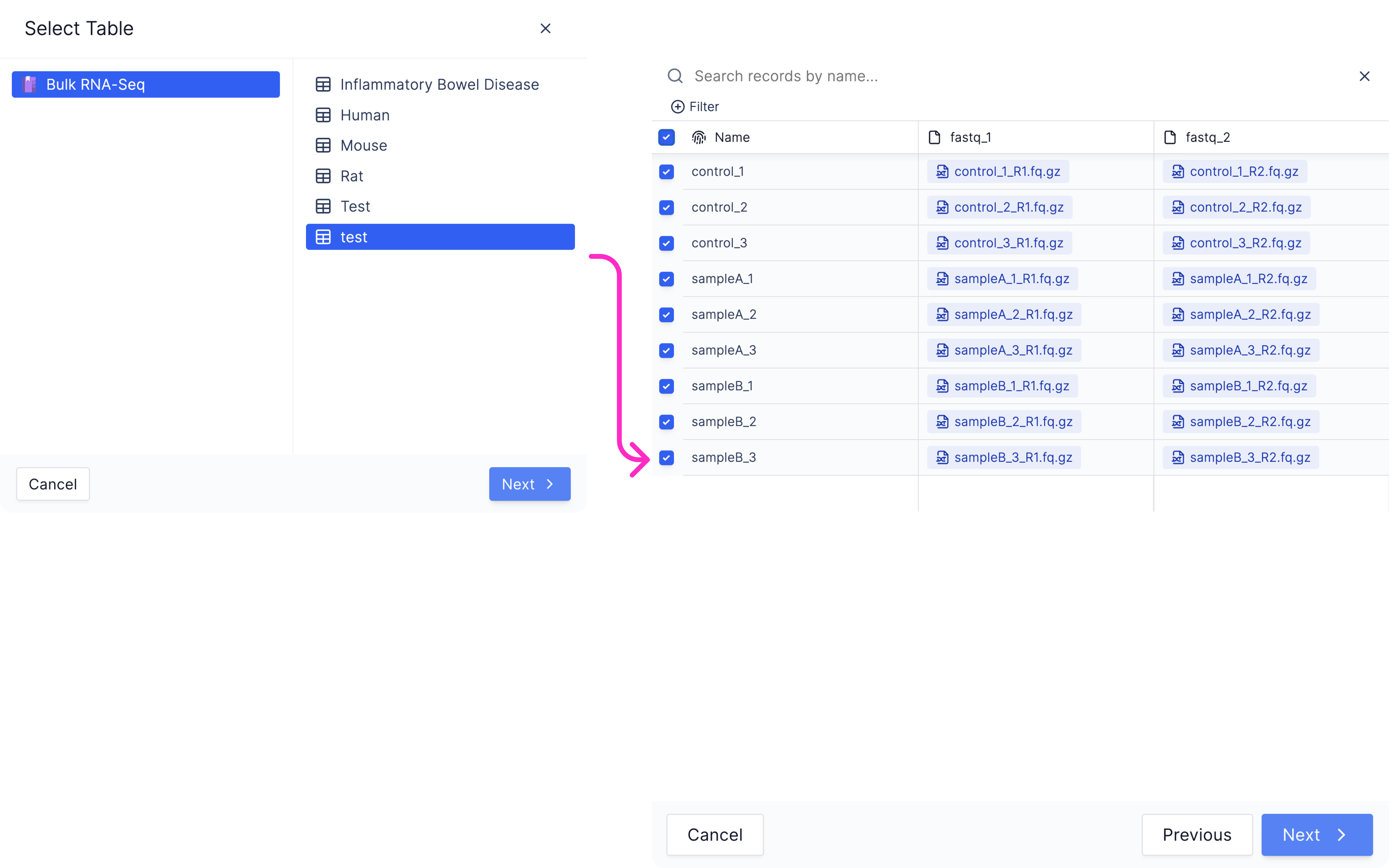
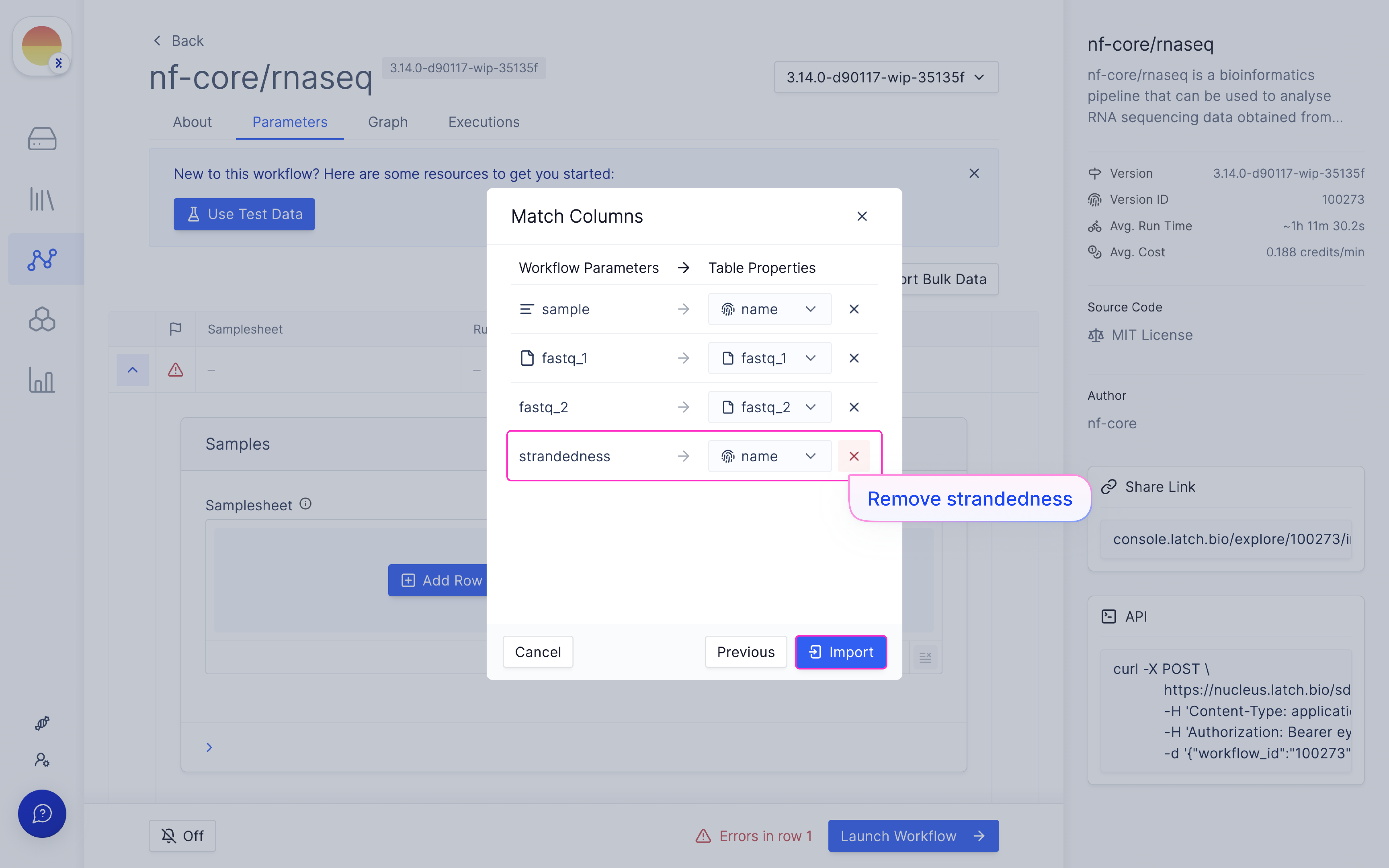
Map samplesheet columns to workflow parameters and click ‘Import’.
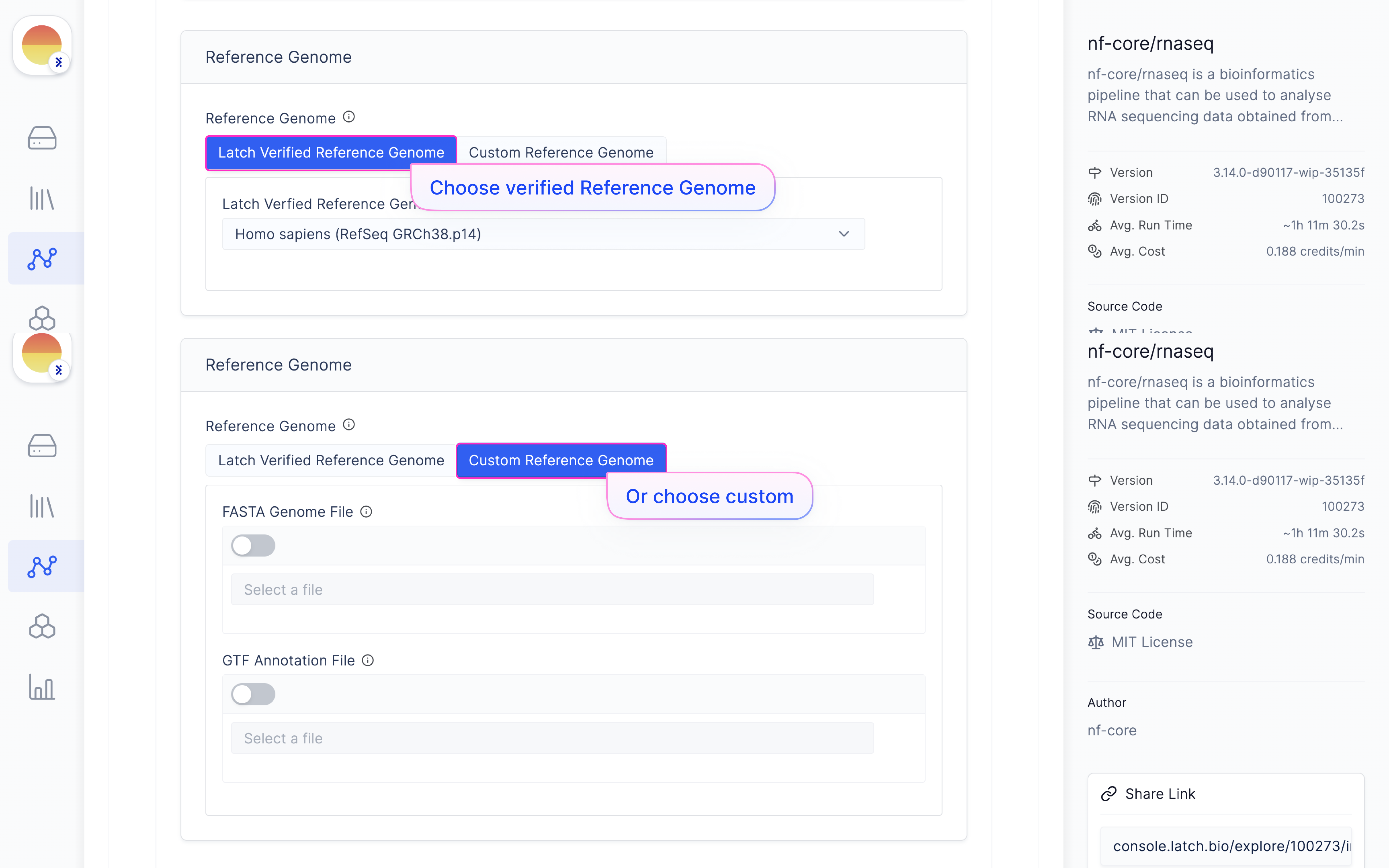
Choose ‘Reference Genome’ from ‘Latch Verified Reference Genome’ tab.
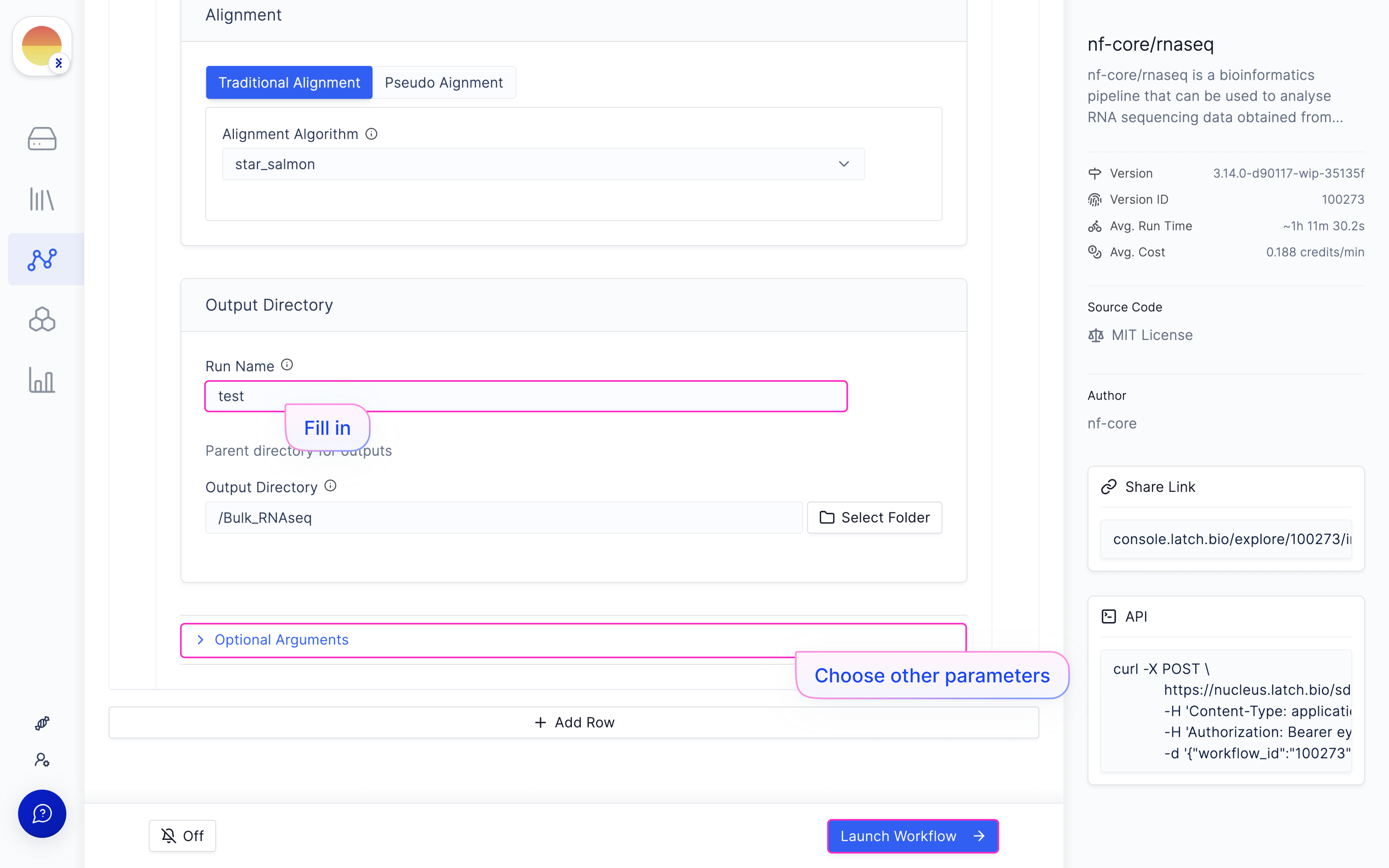
[Fill in a ‘Run Name’ and hit ‘Launch Execution’.
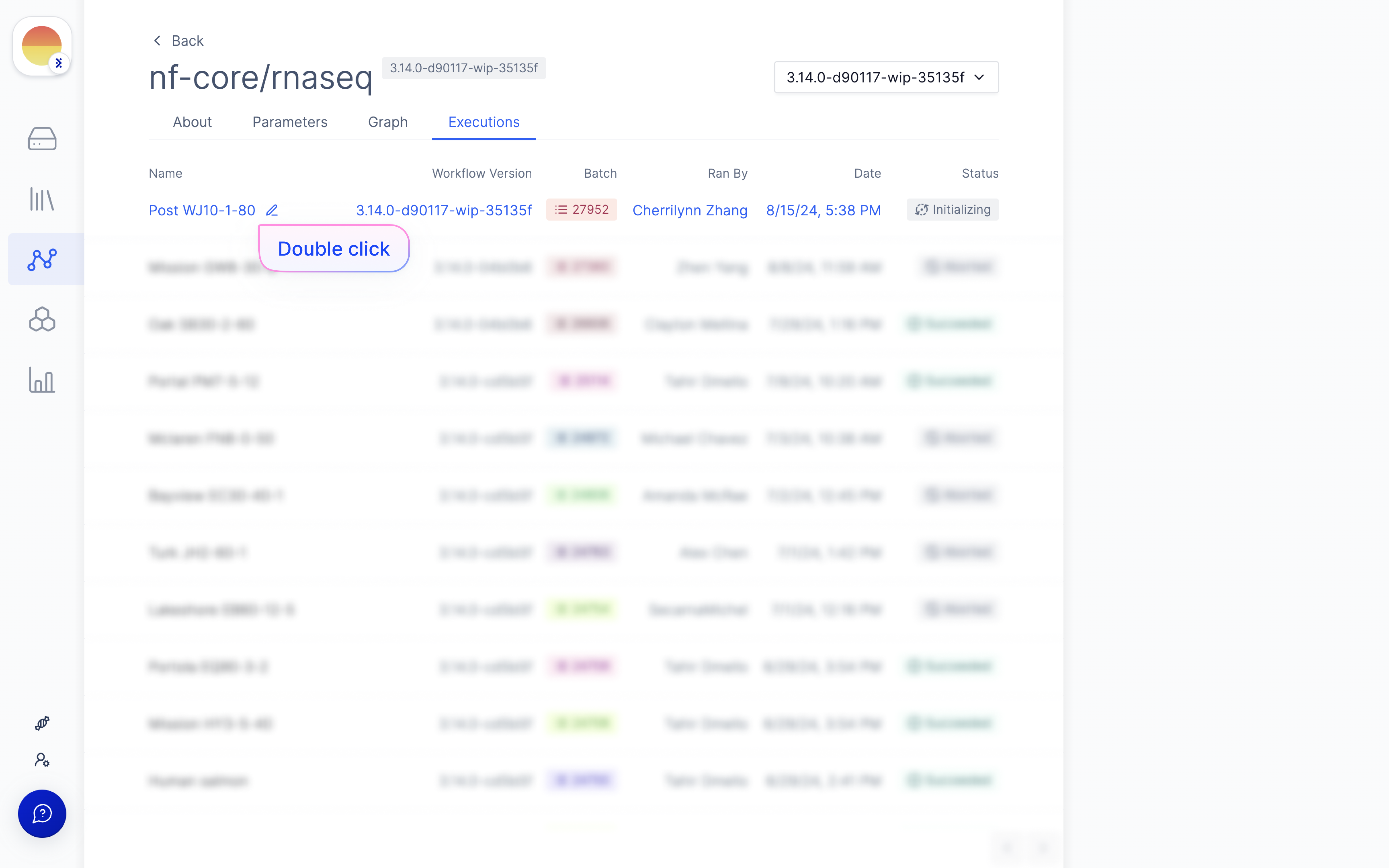
[Optional] Monitor the execution under ‘All Executions’.
Differential Gene Expression
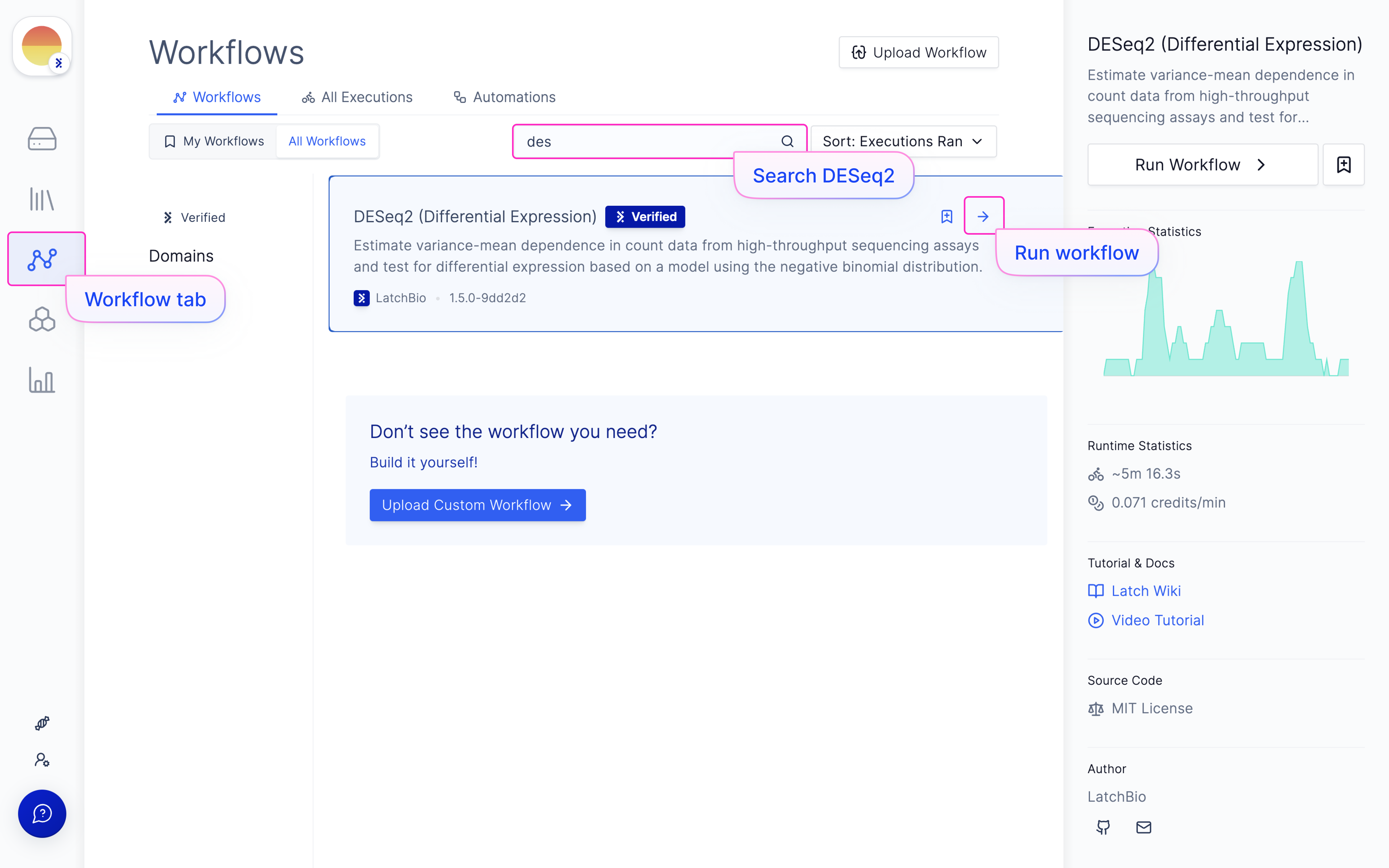
Launch ‘DESeq2 (Differential Expression)’ Latch Workflow
Navigate to the Latch Workflows tab on the left panel.
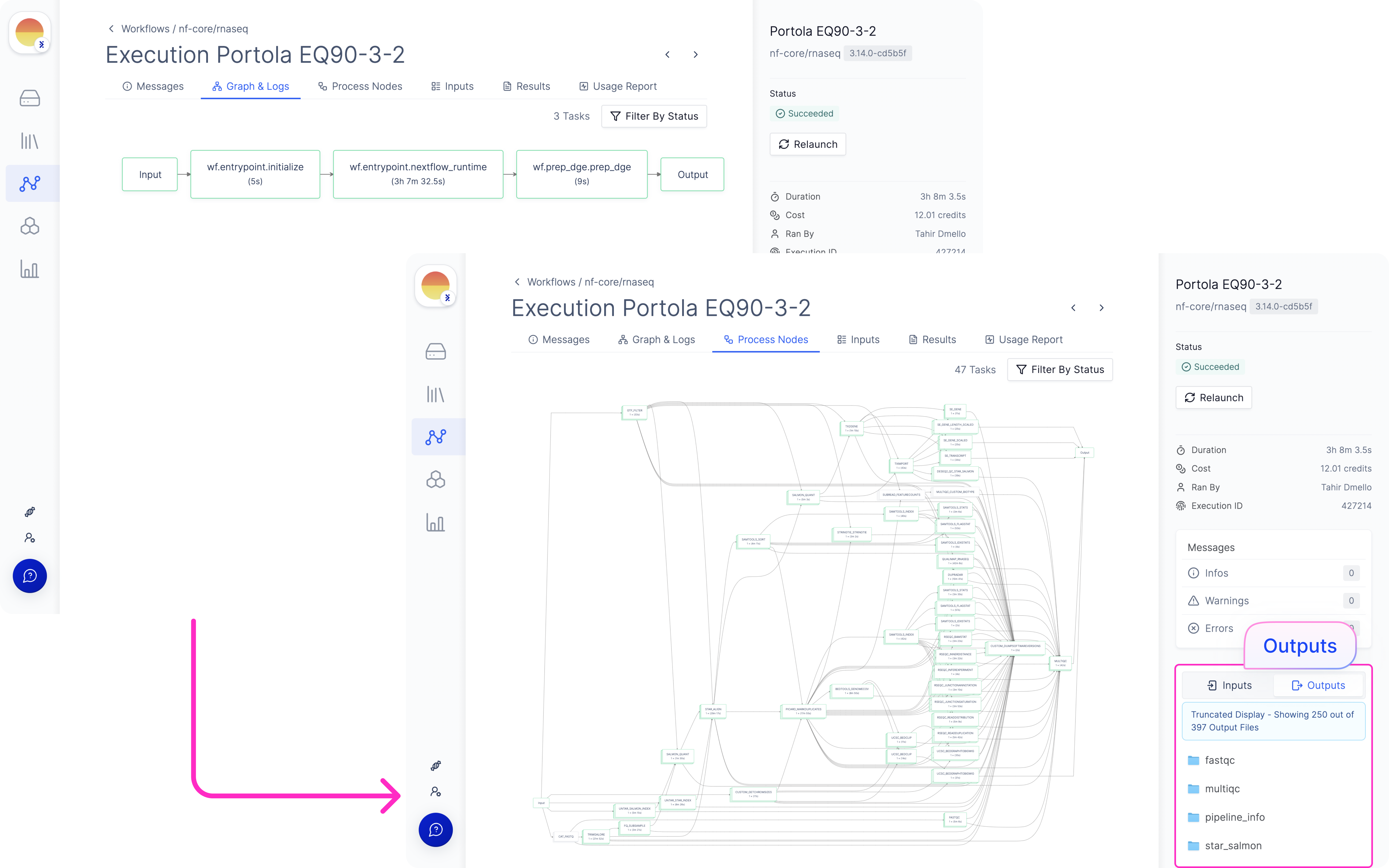
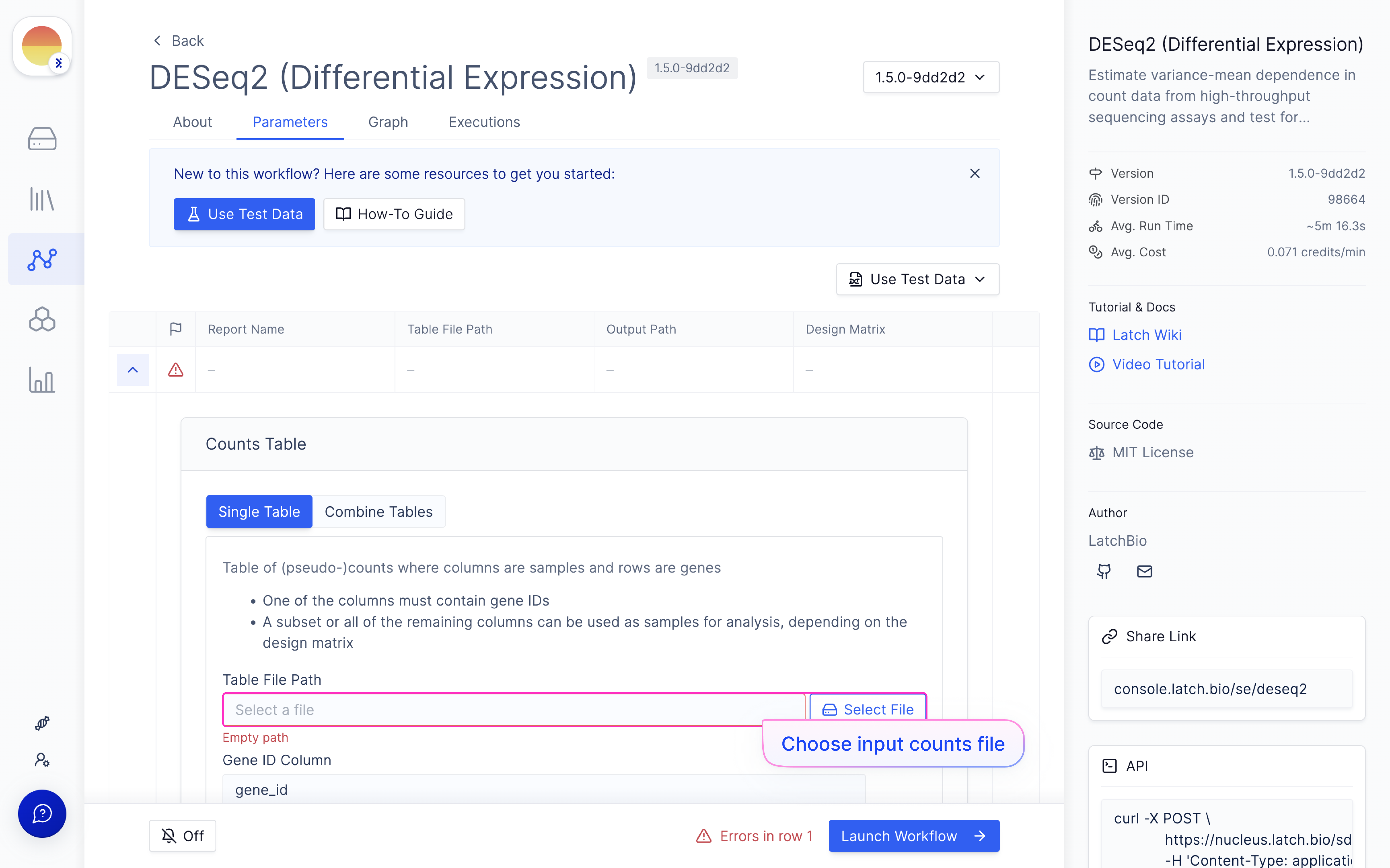
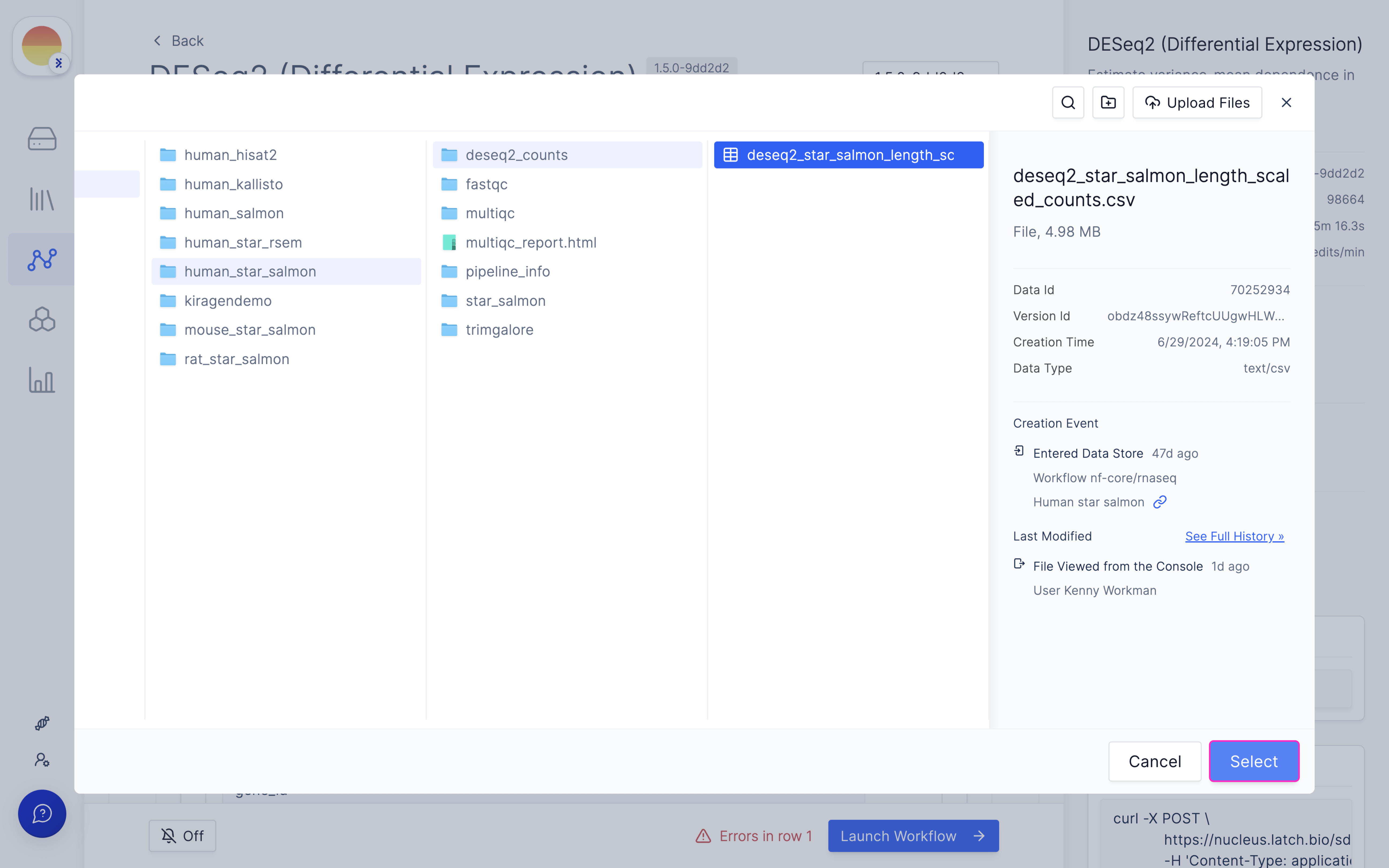
Choose your input counts file from the outputs of ‘nf-core/rnaseq’.
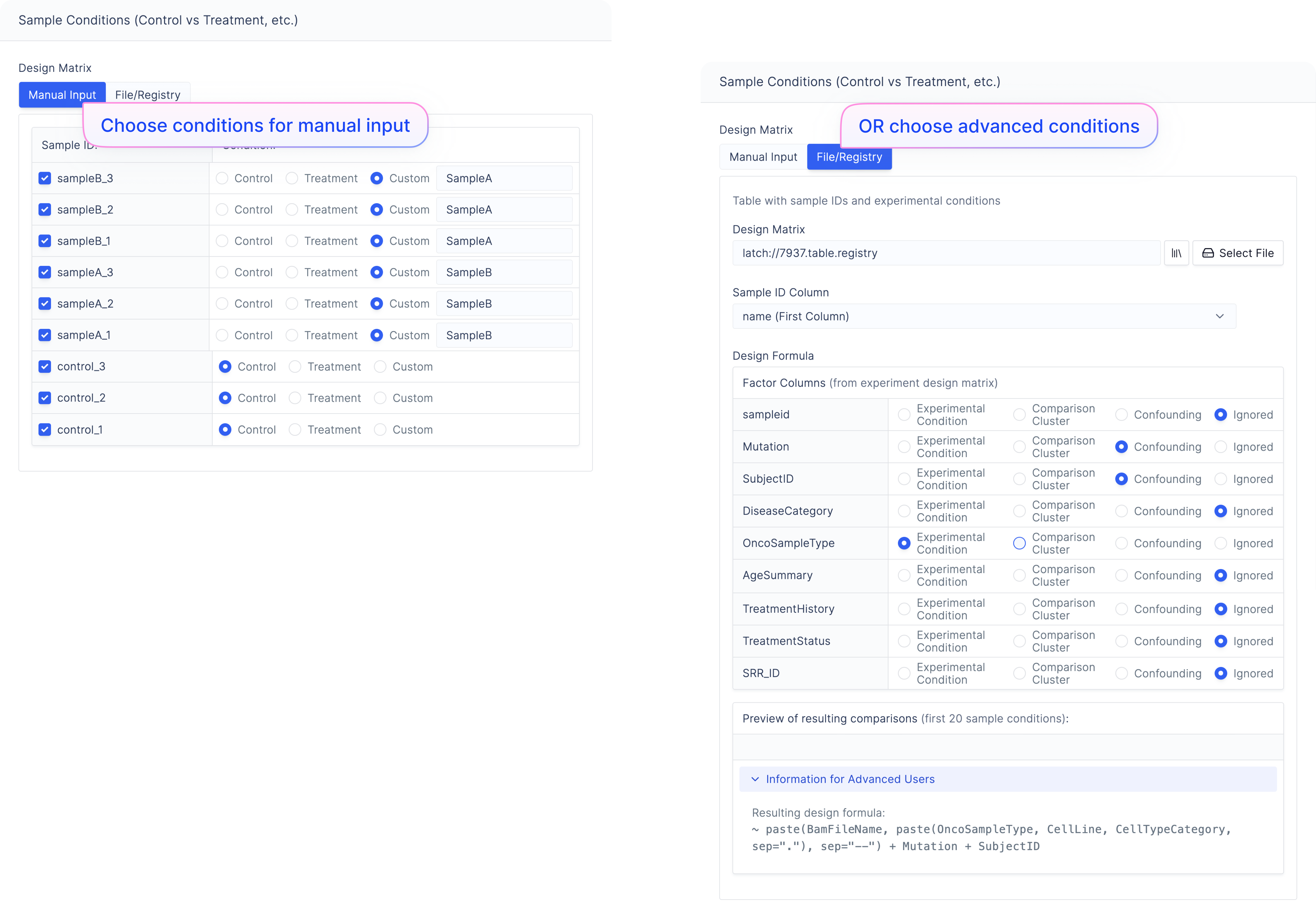
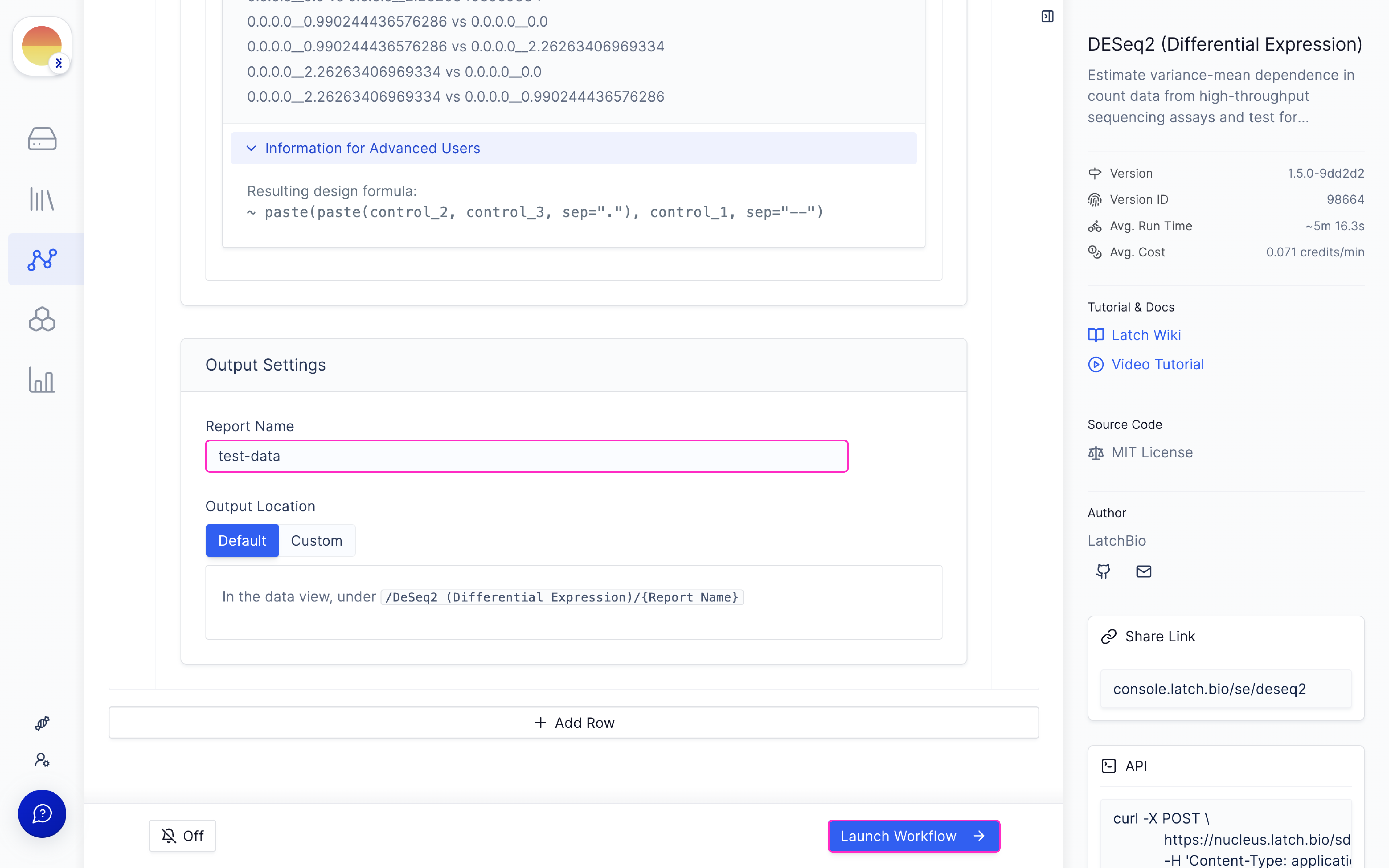
Choose your conditions for your samples in the ‘Manual Input’ design matrix tab.
Visualize differential gene expression outputs in Latch Plots
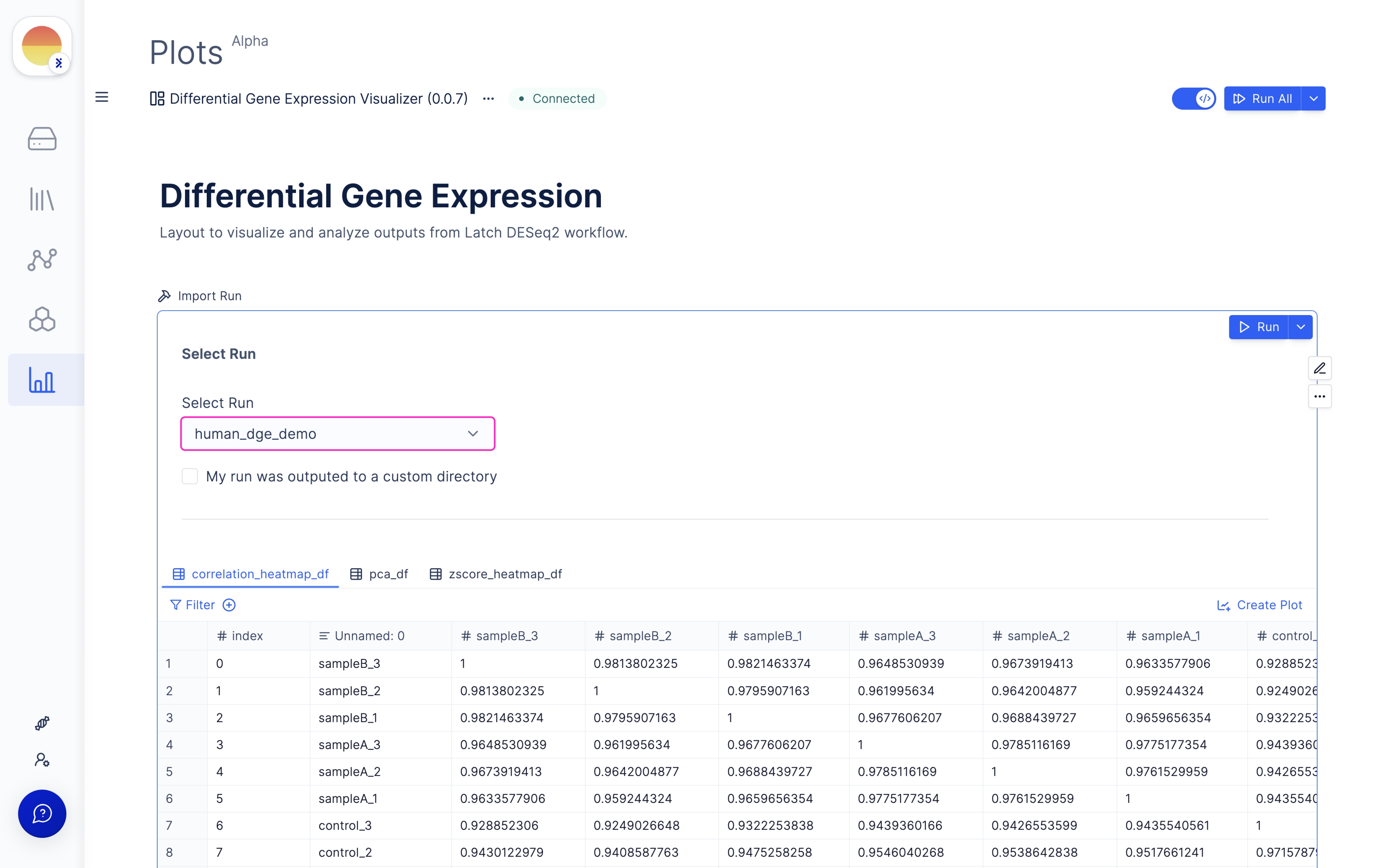
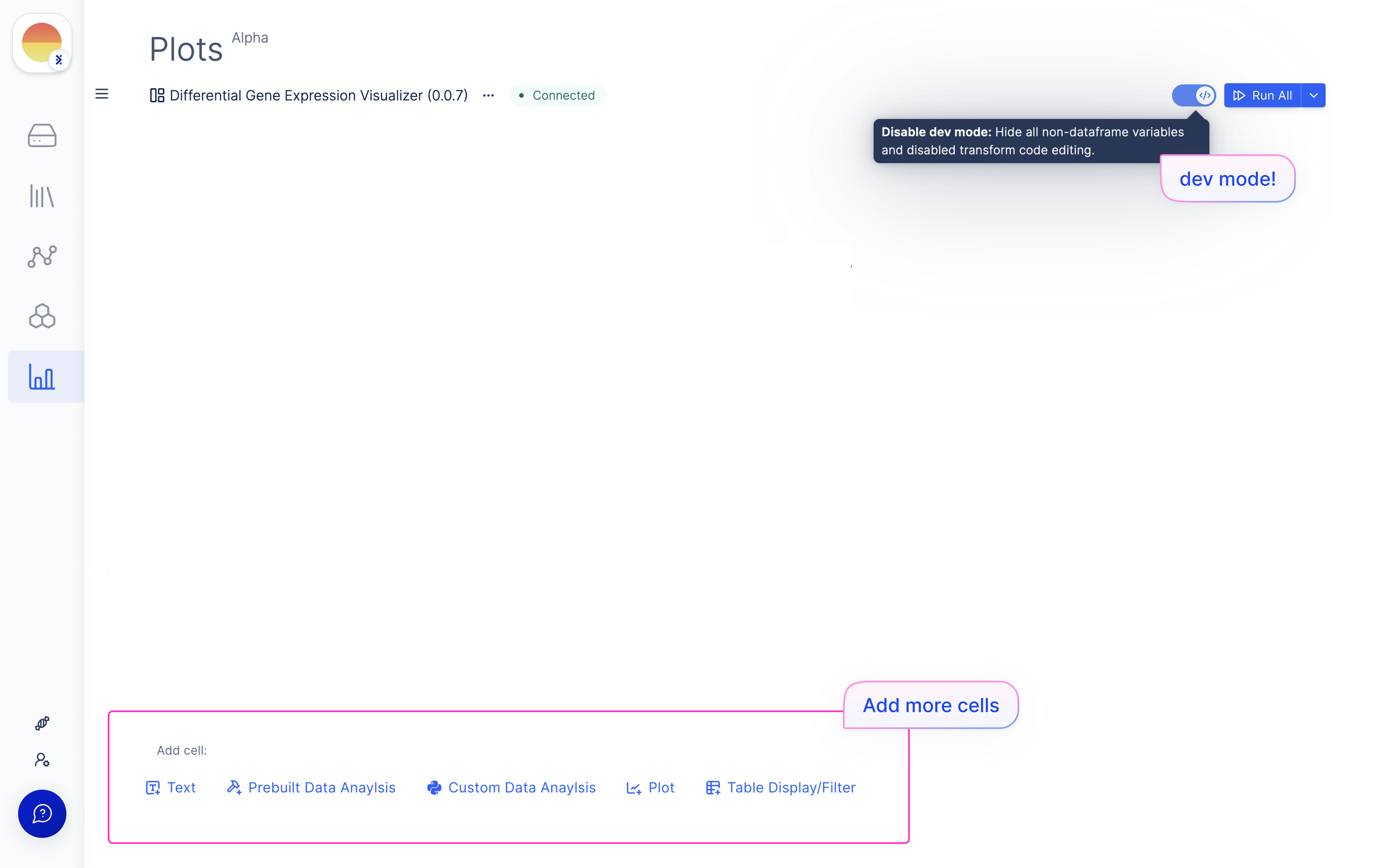
Navigate to the Latch Plots tab on the left panel.
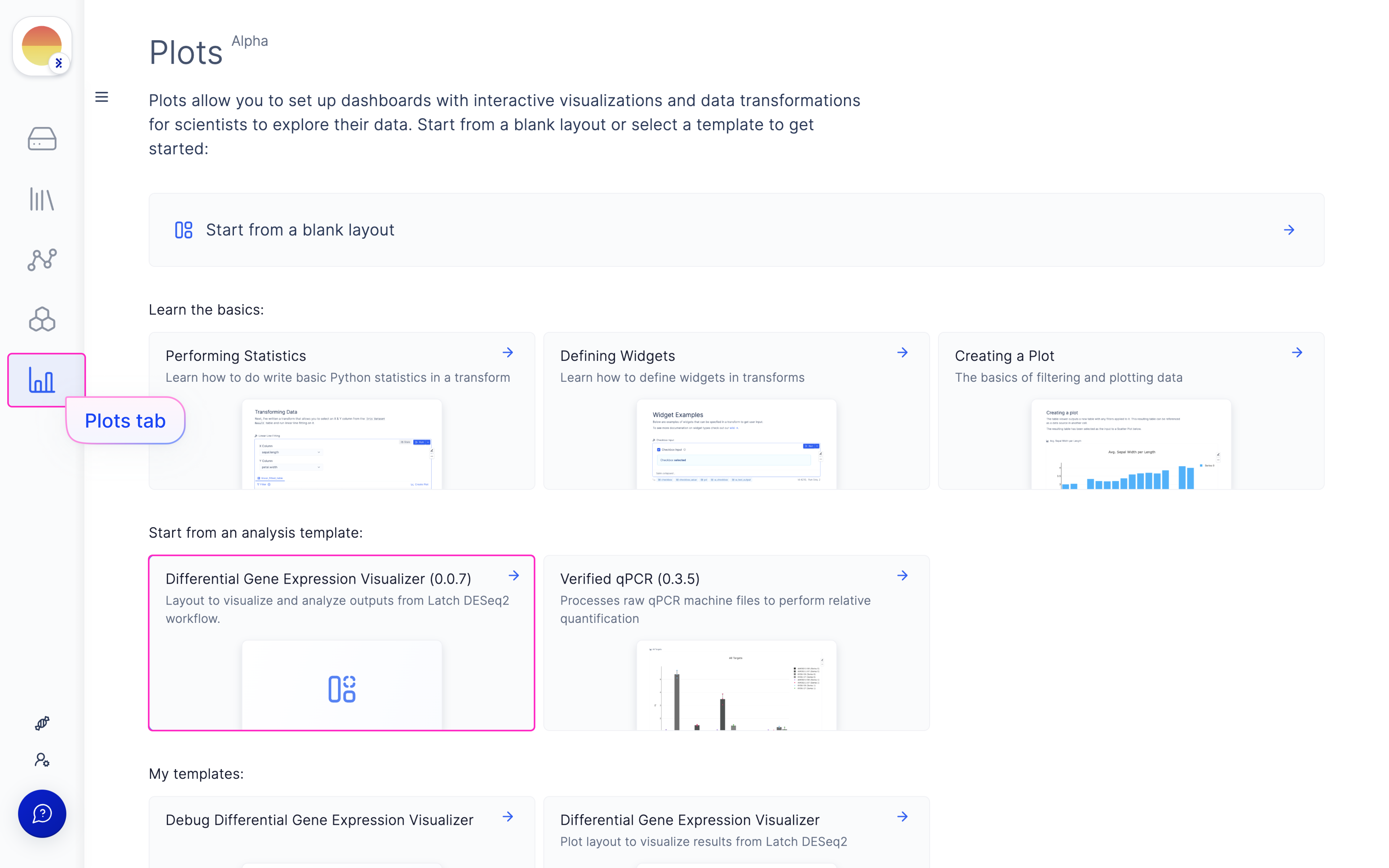
Once the DESeq2 run is done, choose your outputted run (or select from Latch Data if a custom output location was used) and scroll through for QC graphs and heatmaps.
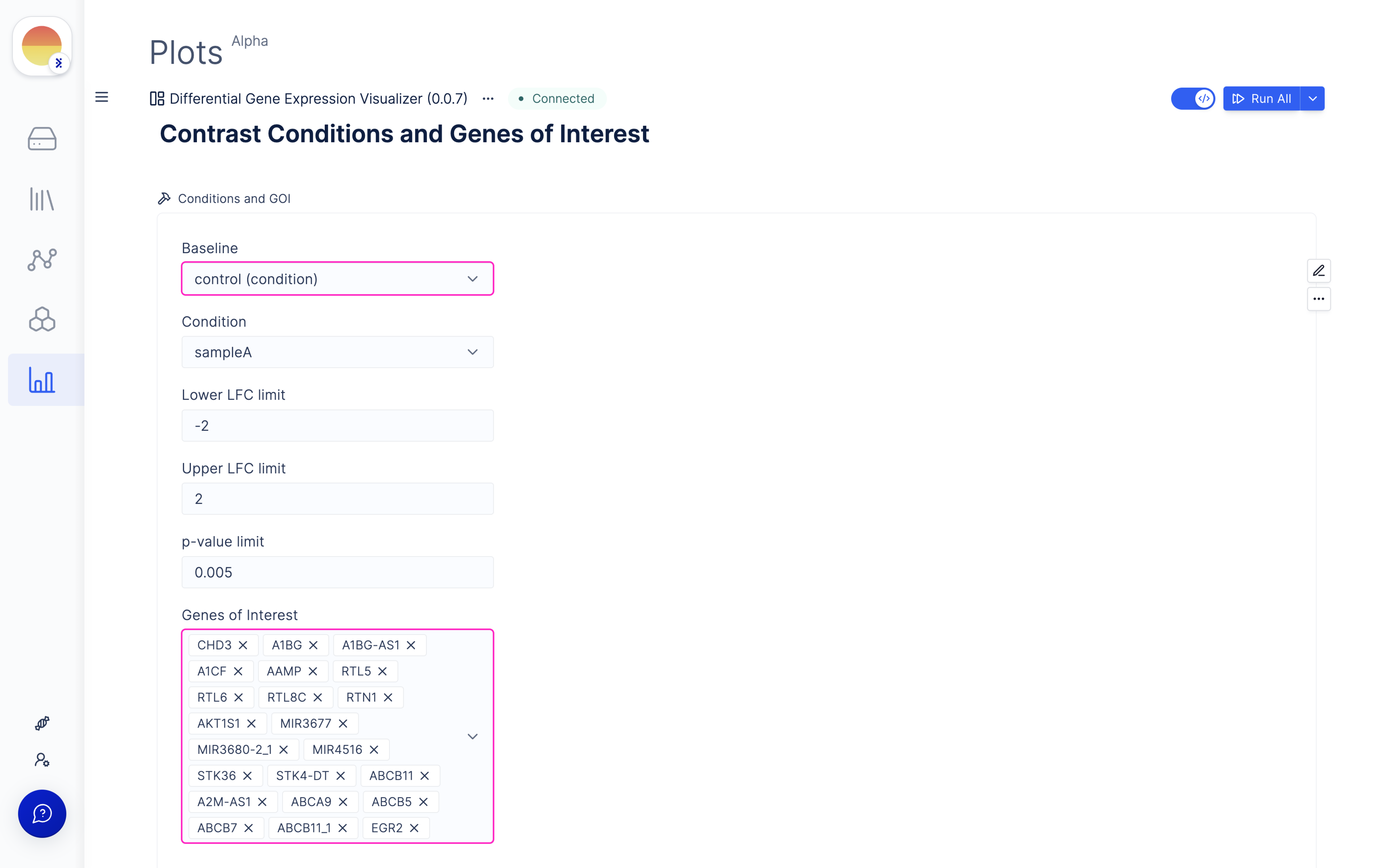
Choose ‘Contrast Conditions’ and ‘Genes of Interest’ for comparison and visualize Volcano and MA Plots.
Pathway Enrichment
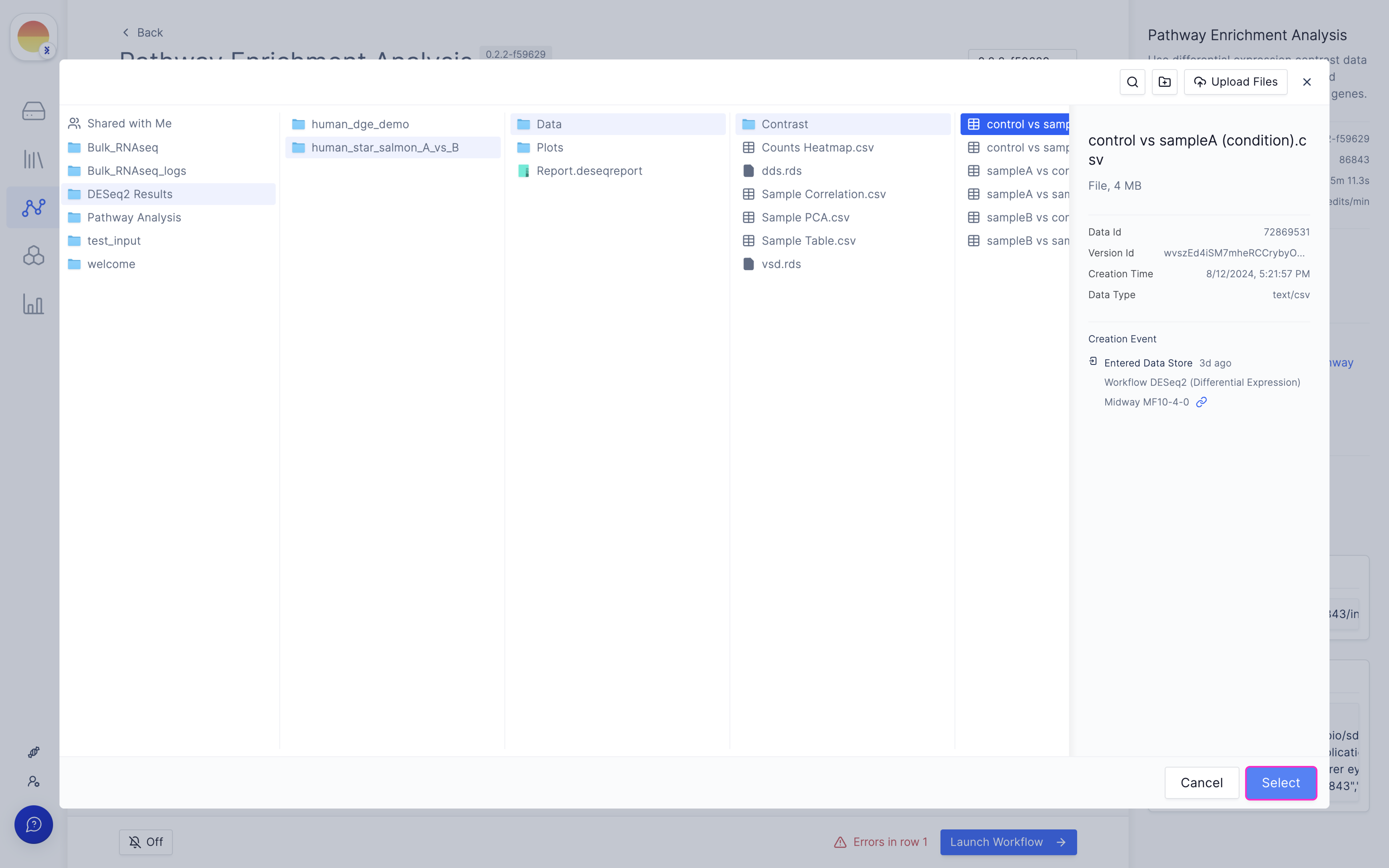
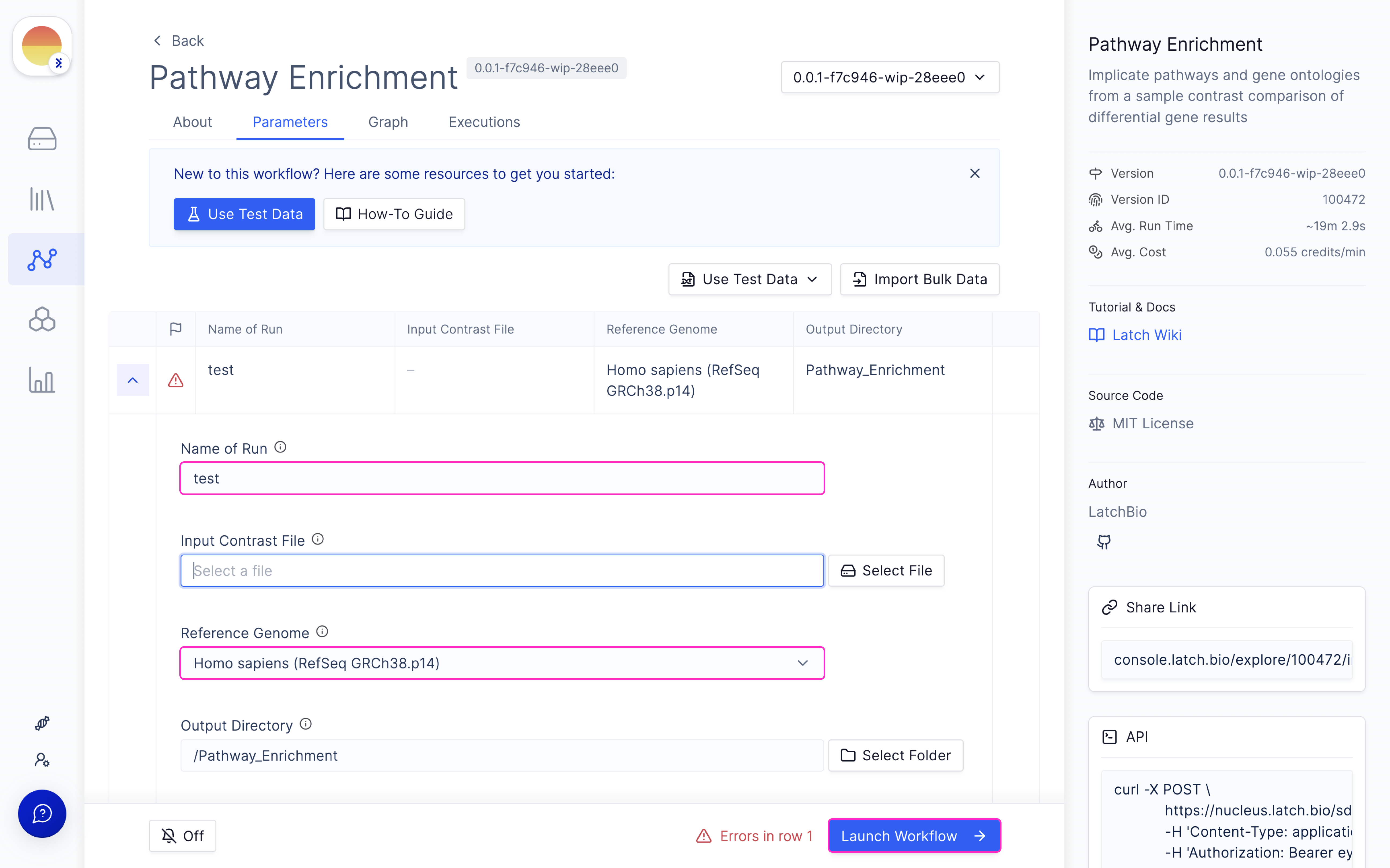
Launch ‘Pathway Enrichment Analysis’ Latch Workflow
Navigate to the Latch Workflows tab on the left panel.
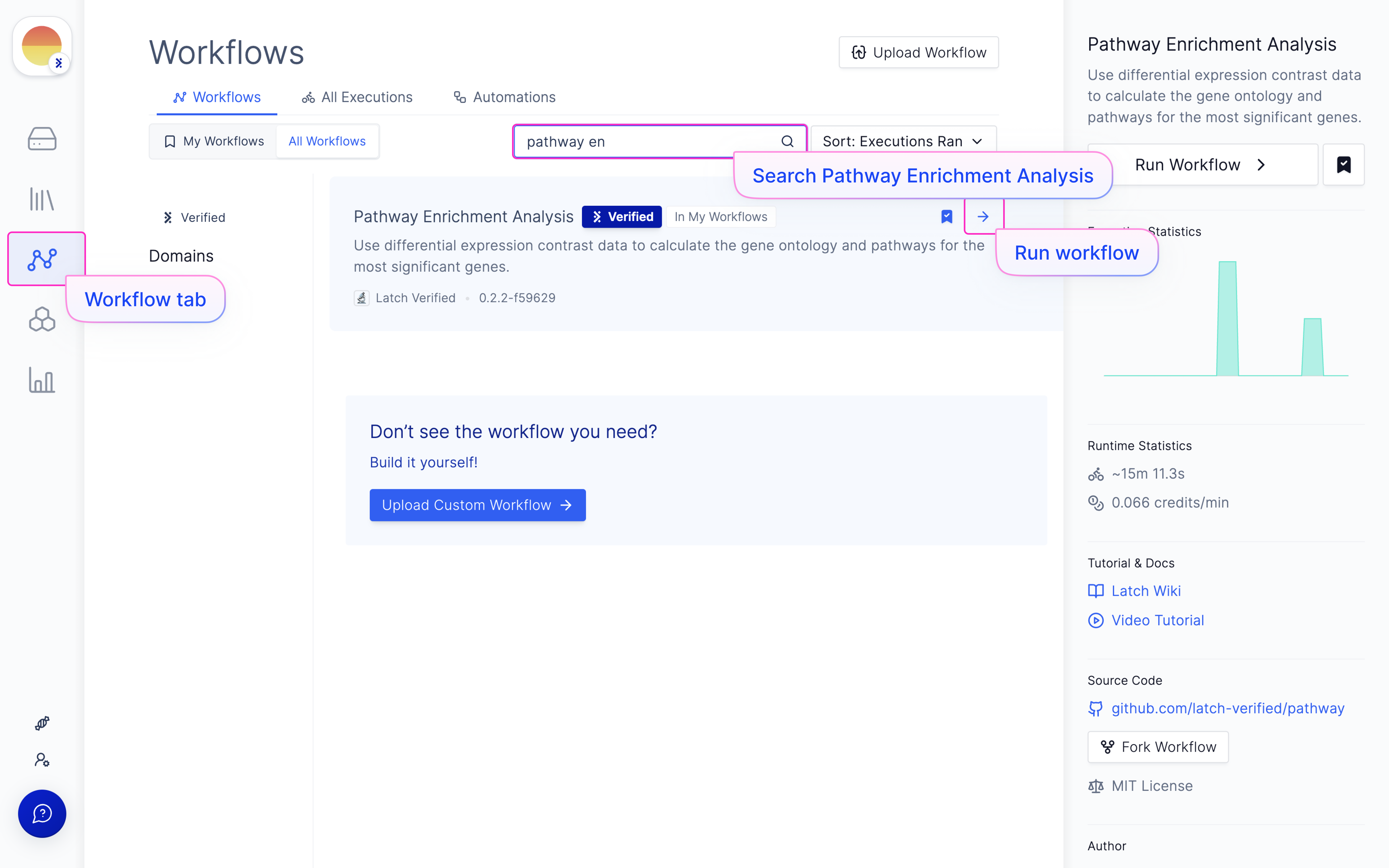
Choose your needed contrast file from the DESeq2 run output.